MTH028 Linear Algebra I - Lecture Notes

Author

Jiaye Xu

Published

September 3, 2026

Chapter 1 Linear Equations in Linear Algebra

Section 1.1 Systems of Linear Equations

Learning Objectives

After this lecture you will be able to:

Recognize a linear equation and a system of linear equations.
Explain what a solution of a linear system is and describe the geometric meaning of a system of two equations.
Write a linear system in matrix notation (coefficient matrix, augmented matrix).
Use elementary row operations to produce an equivalent system.
Determine whether a system is consistent and whether a solution is unique by looking at the augmented matrix in (near‑)triangular form.

What is a linear equation?

A linear equation in the variables \(x_1, x_2, \dots, x_n\) is an equation that can be written as

\[a_1 x_1 + a_2 x_2 + \cdots + a_n x_n = b \qquad\qquad (1)\]

where \(b\) and the coefficients \(a_1, \dots, a_n\) are real (or complex) numbers known in advance.
The subscript \(n\) can be any positive integer. In real‑life problems \(n\) may be 50, 5000, or even larger.

Which of the following are linear?

\(4x_1 - 5x_2 + 2 = x_1\)
→ rearranges to \(3x_1 - 5x_2 = -2\) (linear)
\(x_2 = 2(\sqrt{6} - x_1) + x_3\)
→ rearranges to \(2x_1 + x_2 - x_3 = 2\sqrt{6}\) (linear)
\(4x_1 - 5x_2 = x_1 x_2\) (product \(x_1 x_2\) → not linear)
\(x_2 = 2\sqrt{x_1} - 6\) (square root → not linear)

Systems of linear equations

A system of linear equations (or linear system) is a collection of one or more linear equations in the same variables.
For example,

\[\begin{aligned} 2x_1 - x_2 + 1.5x_3 &= 8 \\ x_1 - 4x_3 &= -7 \end{aligned} \qquad\qquad (2)\]

A solution of the system is a list \((s_1, s_2, \dots, s_n)\) that makes every equation true when substituted for \(x_1, \dots, x_n\).
The solution set is the set of all possible solutions.

Two systems are equivalent if they have the same solution set.

Geometric interpretation (two variables)

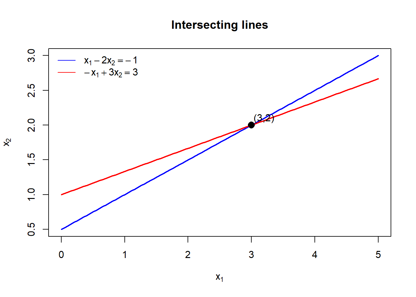
A system of two equations in two unknowns corresponds to two lines in the plane.
The solution set is the intersection of these lines. Three possibilities exist:

Exactly one solution – the lines intersect at a single point.
No solution – the lines are parallel (and distinct).
Infinitely many solutions – the lines coincide (are the same line).

The textbook illustrations (Figures 1 and 2) show these cases. We can reproduce them with R.

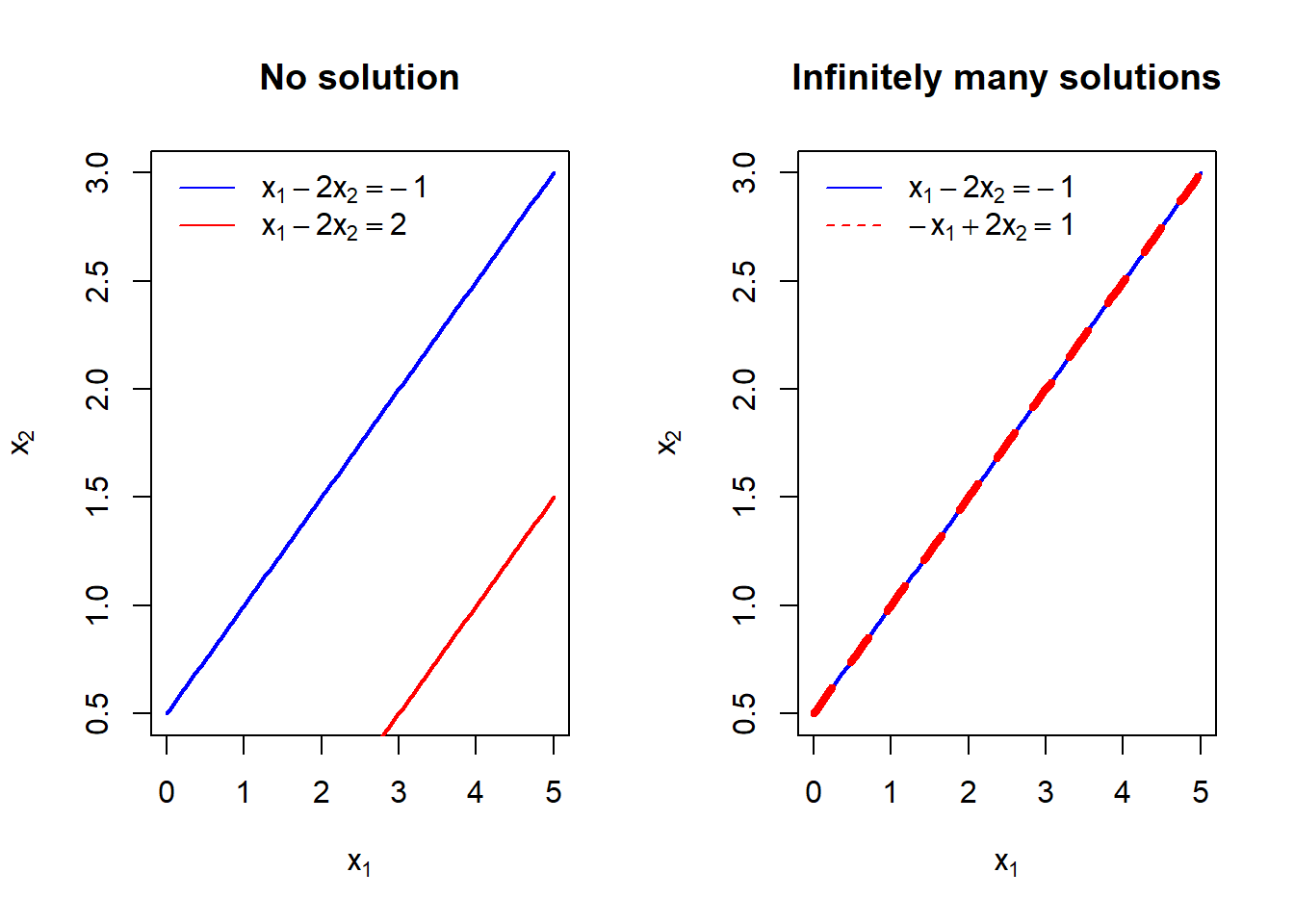
Two lines crossing at the point (3,2) — Exactly one solution: lines intersect at (3,2)

Two plots; left two parallel lines, right one line over another. — Left: parallel lines (no solution). Right: coincident lines (infinitely many solutions).

Take‑away: A linear system can have no solution, exactly one solution, or infinitely many solutions.

A system is consistent if it has at least one solution; it is inconsistent if it has no solution.

Matrix notation

The essential information of a system can be stored in a rectangular array called a matrix.
For the system

\[\begin{aligned} x_1 - 2x_2 + x_3 &= 0 \\ 2x_2 - 8x_3 &= 8 \\ 5x_1 - 5x_3 &= 10 \end{aligned} \qquad\quad (3)\]

Coefficient matrix

\[\begin{bmatrix} 1 & -2 & 1 \\ 0 & 2 & -8 \\ 5 & 0 & -5 \end{bmatrix}\]

Augmented matrix (coefficients + right‑hand side)

\[\left[\begin{array}{rrr|r} 1 & -2 & 1 & 0 \\ 0 & 2 & -8& 8 \\ 5 & 0 & -5& 10 \end{array}\right] \qquad\quad (4)\]

The augmented matrix is a \(3 \times 4\) matrix (3 rows, 4 columns).
We always write the number of rows first.

Elementary row operations

To solve a system we replace it with an equivalent system that is easier to handle.
Three operations on the augmented matrix do not change the solution set:

Replacement – replace one row by the sum of itself and a multiple of another row.
Interchange – swap two rows.
Scaling – multiply all entries of a row by a nonzero constant.

These are called elementary row operations. They are reversible:

Interchange again to undo.
If scaled by \(c \neq 0\), multiply by \(1/c\).
If row 2 is replaced by \(\text{row}_2 + c\cdot\text{row}_1\), adding \(-c\cdot\text{row}_1\) to the new row 2 restores the original.

Two matrices are row equivalent if there is a sequence of row operations that transforms one into the other.

Important fact: If the augmented matrices of two linear systems are row equivalent, then the two systems have the same solution set.

Solving a linear system – Example 1 (textbook)

We solve system (3) using row operations on the augmented matrix.
The steps are shown with both the equation form and the matrix form.

Operation	Resulting system (equations)	Augmented matrix
Original system	\(\begin{aligned} x_1-2x_2+x_3&=0 \\ 2x_2-8x_3&=8 \\ 5x_1-5x_3&=10 \end{aligned}\)	\(\left[\begin{array}{rrr\\|r}1&-2&1&0\\0&2&-8&8\\5&0&-5&10\end{array}\right]\)
Eliminate \(x_1\) in eq.3: \(\text{eq3} -5\cdot\text{eq1}\)	\(\begin{aligned} x_1-2x_2+x_3&=0 \\ 2x_2-8x_3&=8 \\ 10x_2-10x_3&=10 \end{aligned}\)	\(\left[\begin{array}{rrr\\|r}1&-2&1&0\\0&2&-8&8\\0&10&-10&10\end{array}\right]\)
Scale eq.2 by \(\frac12\)	\(\begin{aligned} x_1-2x_2+x_3&=0 \\ x_2-4x_3&=4 \\ 10x_2-10x_3&=10 \end{aligned}\)	\(\left[\begin{array}{rrr\\|r}1&-2&1&0\\0&1&-4&4\\0&10&-10&10\end{array}\right]\)
Eliminate \(x_2\) in eq.3: \(\text{eq3} -10\cdot\text{eq2}\)	\(\begin{aligned} x_1-2x_2+x_3&=0 \\ x_2-4x_3&=4 \\ 30x_3&=-30 \end{aligned}\)	\(\left[\begin{array}{rrr\\|r}1&-2&1&0\\0&1&-4&4\\0&0&30&-30\end{array}\right]\)
Scale eq.3 by \(\frac{1}{30}\)	\(\begin{aligned} x_1-2x_2+x_3&=0 \\ x_2-4x_3&=4 \\ x_3&=-1 \end{aligned}\)	\(\left[\begin{array}{rrr\\|r}1&-2&1&0\\0&1&-4&4\\0&0&1&-1\end{array}\right]\)
Back‑substitute: use \(x_3\) to clean rows above	\(\begin{aligned} x_1-2x_2 &= 1 \\ x_2 &= 0 \\ x_3 &= -1 \end{aligned}\)	\(\left[\begin{array}{rrr\\|r}1&-2&0&1\\0&1&0&0\\0&0&1&-1\end{array}\right]\)
Eliminate \(-2x_2\) in eq.1	\(\begin{aligned} x_1 &= 1 \\ x_2 &= 0 \\ x_3 &= -1 \end{aligned}\)	\(\left[\begin{array}{rrr\\|r}1&0&0&1\\0&1&0&0\\0&0&1&-1\end{array}\right]\)

The solution is \((x_1, x_2, x_3) = (1, 0, -1)\).

This example illustrates how operations on equations in a linear system correspond to operations on the appropriate rows of the augmented matrix.
Each original equation represents a plane in \(\mathbb{R}^3\), and these three planes intersect at exactly the point \((1,0,-1)\).

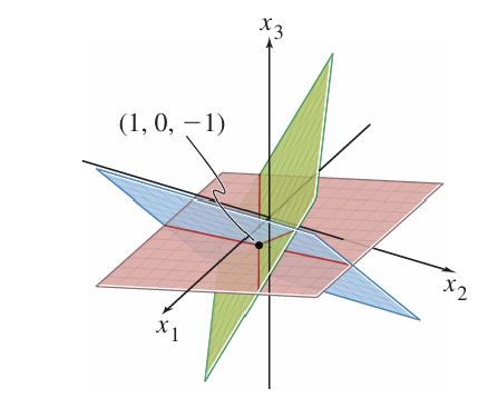
(Textbook Figure for Example 1: three planes intersecting at (1,0,-1).)

Existence and uniqueness questions

When we reduce a system to a triangular (or nearly triangular) form, we can quickly answer two fundamental questions:

Is the system consistent? (Does at least one solution exist?)

If a solution exists, is it unique?

Example 2 – Consistent, unique solution

The system from Example 1 after the forward elimination step (just before back‑substitution) gave the triangular form

\[\left[\begin{array}{rrr|r} 1 & -2 & 1 & 0 \\ 0 & 1 & -4 & 4 \\ 0 & 0 & 1 & -1 \end{array}\right]\]

There is no row of the form \([0\;0\;0\;| \;b]\) with \(b\neq0\), so a solution exists.
From the third equation we obtain \(x_3\), then back‑substitution gives unique values for \(x_2\) and \(x_1\).
The solution is unique.

Example 3 – Inconsistent system

Consider the system (textbook Example 3)

\[\begin{aligned} x_2 - 4x_3 &= 8 \\ 2x_1 - 3x_2 + 2x_3 &= 1 \\ 4x_1 - 8x_2 + 12x_3 &= 1 \end{aligned} \qquad\quad (5)\]

Augmented matrix:

\[\left[\begin{array}{rrr|r} 0 & 1 & -4 & 8 \\ 2 & -3 & 2 & 1 \\ 4 & -8 & 12 & 1 \end{array}\right]\]

Step 1: Interchange row1 and row2 to get a nonzero leading entry (the leftmost nonzero entry of a row) in column 1.

\[\left[\begin{array}{rrr|r} 2 & -3 & 2 & 1 \\ 0 & 1 & -4 & 8 \\ 4 & -8 & 12 & 1 \end{array}\right]\]

Step 2: Eliminate \(4x_1\) in row3: \(\text{row3} \leftarrow \text{row3} - 2\cdot\text{row1}\).

\[\left[\begin{array}{rrr|r} 2 & -3 & 2 & 1 \\ 0 & 1 & -4 & 8 \\ 0 & -2 & 8 & -1 \end{array}\right]\]

Step 3: Eliminate \(-2x_2\) in row3: \(\text{row3} \leftarrow \text{row3} + 2\cdot\text{row2}\).

\[\left[\begin{array}{rrr|r} 2 & -3 & 2 & 1 \\ 0 & 1 & -4 & 8 \\ 0 & 0 & 0 & 15 \end{array}\right] \qquad\quad (7)\]

The last row reads \(0x_1 + 0x_2 + 0x_3 = 15\), which is impossible.
The system is inconsistent – no solution exists.

Comments: In matrix language, the rightmost column of the augmented matrix is a pivot column, which signals inconsistency. (details in the following section)
From the geometric perspective, the system is inconsistent because there is no point that lies on all three planes.

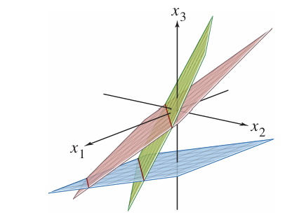
(Textbook Figure for Example 3: three planes that have no common intersection.)

Numerical note (brief)

In real-world problems, systems of linear equations are solved by a computer. For a square coefficient matrix, computers use the elimination algorithm given here and later in Section1.2, modified slightly for improved accuracy.

When systems are solved by computers, arithmetic is performed with floating point numbers (about 8–16 decimal digits). Small round‑off errors can occur, but they rarely cause problems in well‑conditioned problems. The row‑reduction algorithm used in practice selects pivots with the largest absolute value (partial pivoting) to improve accuracy.

Practice problems (in‑class)

Try these yourself before looking at the solutions.

Write the augmented matrix of the system

\[\begin{aligned} x_1 + 4x_2 - 2x_3 + 8x_4 &= 12 \\ x_2 - 7x_3 + 2x_4 &= -4 \\ 5x_3 - x_4 &= 7 \\ x_3 + 3x_4 &= -5 \end{aligned}\]

Then state the next elementary row operation that should be performed to solve it.
The augmented matrix of a linear system has been reduced to

\[\left[\begin{array}{rrrr|r} 1 & 0 & 0 & 0 & 2 \\ 0 & 1 & 0 & 2 & 3 \\ 0 & 0 & 1 & -1 & 5 \end{array}\right]\]

Is the system consistent? If so, is the solution unique?
Is \((3,4,-2)\) a solution of

\[\begin{aligned} 5x_1 - x_2 + 2x_3 &= 7 \\ -2x_1 + 6x_2 + 9x_3 &= 0 \\ -7x_1 + 5x_2 - 3x_3 &= -7 \end{aligned}?\]
For what values of \(h\) and \(k\) is the system

\[\begin{aligned} 2x_1 - x_2 &= h \\ -6x_1 + 3x_2 &= k \end{aligned}\]

consistent?

(Solutions are provided at the end of the notes.)

R supplement: row reduction

You can perform elementary row operations in R exactly as we did by hand.
Here is the code for Example 1:

# Augmented matrix for Example 1
A <- matrix(c(1, -2,  1,  0,
              0,  2, -8,  8,
              5,  0, -5, 10), nrow=3, byrow=TRUE)
A

     [,1] [,2] [,3] [,4]
[1,]    1   -2    1    0
[2,]    0    2   -8    8
[3,]    5    0   -5   10

# Forward elimination
A[3,] <- A[3,] - 5*A[1,]   # eliminate x1 in row3
A[2,] <- A[2,] / 2          # scale row2
A[3,] <- A[3,] - 10*A[2,]   # eliminate x2 in row3
A[3,] <- A[3,] / 30         # scale row3
A

     [,1] [,2] [,3] [,4]
[1,]    1   -2    1    0
[2,]    0    1   -4    4
[3,]    0    0    1   -1

# Backward elimination (create reduced echelon form)
A[2,] <- A[2,] + 4*A[3,]    # clean above pivot in col3
A[1,] <- A[1,] - 1*A[3,]
A[1,] <- A[1,] + 2*A[2,]    # clean above pivot in col2
A

     [,1] [,2] [,3] [,4]
[1,]    1    0    0    1
[2,]    0    1    0    0
[3,]    0    0    1   -1

The final matrix shows \(x_1=1\), \(x_2=0\), \(x_3=-1\).

You can also check consistency quickly. For Example 3:

B <- matrix(c(0, 1, -4,  8,
              2, -3, 2,  1,
              4, -8, 12, 1), nrow=3, byrow=TRUE)
# swap rows 1 and 2
B[c(1,2),] <- B[c(2,1),]
# eliminate below first pivot
B[3,] <- B[3,] - 2*B[1,]
# eliminate below second pivot
B[3,] <- B[3,] + 2*B[2,]
B

     [,1] [,2] [,3] [,4]
[1,]    2   -3    2    1
[2,]    0    1   -4    8
[3,]    0    0    0   15

The row 0 0 0 15 indicates an inconsistent system.

Solutions to practice problems

Augmented matrix:

\[\left[\begin{array}{rrrr|r} 1 & 4 & -2 & 8 & 12 \\ 0 & 1 & -7 & 2 & -4 \\ 0 & 0 & 5 & -1& 7 \\ 0 & 0 & 1 & 3& -5 \end{array}\right]\]

A good next operation: interchange row3 and row4 to bring a “1” into the third pivot position (or scale row3 by \(1/5\)).
The system is consistent (no row \([0\;0\;0\;0\;b]\) with \(b\neq0\)). The pivot columns are 1,2,3; \(x_4\) is free. Therefore the solution is not unique (infinitely many solutions).
Substitute \(x_1=3\), \(x_2=4\), \(x_3=-2\):

Equation 1: \(5(3)-4+2(-2)=15-4-4=7\) ✓
Equation 2: \(-2(3)+6(4)+9(-2) = -6+24-18=0\) ✓
Equation 3: \(-7(3)+5(4)-3(-2) = -21+20+6 = 5 \neq -7\) ✗

\((3,4,-2)\) is not a solution.
Write the augmented matrix and reduce:

\[\left[\begin{array}{rr|r} 2 & -1 & h \\ -6 & 3 & k \end{array}\right]\xrightarrow{\text{row2} + 3\cdot\text{row1}} \left[\begin{array}{rr|r} 2 & -1 & h \\ 0 & 0 & k+3h \end{array}\right]\]

The system is consistent exactly when \(k+3h = 0\) (that is, \(k = -3h\)).
If \(k+3h \neq 0\), the system is inconsistent.

Summary

A linear system can have 0, 1, or infinitely many solutions.
The augmented matrix and elementary row operations preserve the solution set.
Triangular form reveals consistency and uniqueness.
Next week we formalize these ideas into Gaussian elimination and echelon forms.

Section 1.2 Row Reduction and Echelon Forms

Learning Objectives

After this lecture you will be able to:

Distinguish between echelon form and reduced echelon form.
Identify pivot positions and pivot columns in a matrix.
Apply the row reduction algorithm (forward and backward phases) to transform any matrix to its unique reduced echelon form.
Use the reduced echelon form of an augmented matrix to describe all solutions of a linear system, separating basic and free variables.
State the Existence and Uniqueness Theorem and use it to decide whether a system is consistent and, if so, whether the solution is unique.

From last week …

We learned that a linear system can be solved by performing elementary row operations on its augmented matrix.
The operations

Replacement (\(R_i \leftarrow R_i + cR_j\))
Interchange (\(R_i \leftrightarrow R_j\))
Scaling (\(R_i \leftarrow cR_i\), \(c\neq 0\))

produce row equivalent matrices that correspond to equivalent systems.

Today we turn this idea into a precise algorithm and use it to answer the two fundamental questions:

Does a solution exist?

If it exists, is it unique?

Echelon forms

A rectangular matrix is in echelon form (or row echelon form) if it satisfies:

All nonzero rows are above any rows of all zeros.
Each leading entry (the leftmost nonzero entry of a row) is in a column to the right of the leading entry of the row above it.
All entries in a column below a leading entry are zeros.

If, in addition, the following conditions hold, the matrix is in reduced echelon form (or reduced row echelon form, RREF):

The leading entry in each nonzero row is 1.
Each leading 1 is the only nonzero entry in its column.

Examples (adapted from textbook, Example 1).

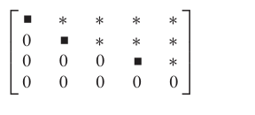
Echelon form (\(\blacksquare\)= any nonzero number, ∗ = any number)

\[\begin{bmatrix} \blacksquare & * & * & * \\ 0 & \blacksquare & * & * \\ 0 & 0 & 0 & 0 \\ 0 & 0 & 0 & 0 \end{bmatrix}\]

,\(\quad\)

\[\begin{bmatrix} 0 & \blacksquare & * & * & * & * & * & * \\ 0 & 0 & 0 & \blacksquare & * & * & * & * \\ 0 & 0 & 0 & 0 & \blacksquare & * & * & * \\ 0 & 0 & 0 & 0 & 0 & 0 & 0 & \blacksquare \end{bmatrix}\]

Reduced echelon form (leading 1s, zeros above and below)

\[\begin{bmatrix} 1 & 0 & * & 0 \\ 0 & 1 & * & 0 \\ 0 & 0 & 0 & 1 \\ 0 & 0 & 0 & 0 \end{bmatrix}\]

,\(\quad\)

\[\begin{bmatrix} 0 & 1 & * & 0 & 0 & * & * & 0 \\ 0 & 0 & 0 & 1 & 0 & * & * & 0 \\ 0 & 0 & 0 & 0 & 1 & * & * & 0 \\ 0 & 0 & 0 & 0 & 0 & 0 & 0 & 1 \end{bmatrix}\]

Comments: Any nonzero matrix may be row reduced (that is,transformed by elementary row operations) into more than one echelon form, using different sequences of row operations (obtaining a row equivalent matrix). However, the reduced echelon form obtained from a matrix is unique.

Theorem 1 (Uniqueness of the Reduced Echelon Form).

Theorem 1: Each matrix is row equivalent to one and only one reduced echelon matrix.

Thus, no matter which sequence of row operations you use, you will always arrive at the same reduced echelon form.

Pivot positions and pivot columns

Definition: A pivot position is a location in a matrix that corresponds to a leading 1 in its reduced echelon form.
A pivot column is a column that contains a pivot position.

Tip

Think of pivot positions as the “stepping‑stones” that determine the shape of the echelon form.

N.B. Locating the pivot positions in an echelon form:

A pivot is the leftmost nonzero entry in an echelon form. Therefore, in Example 1, the squares (\(\blacksquare\)) identify the pivot positions.

Example – Locating pivots (textbook Example 2).
Row reduce the matrix \(A\) below to echelon form and circle the pivot columns.

\[A = \begin{bmatrix} 0 & -3 & -6 & 4 & 9 \\ -1 & -2 & -1 & 3 & 1 \\ -2 & -3 & 0 & 3 & -1 \\ 1 & 4 & 5 & -9 & -7 \end{bmatrix}\]

Step 1. The leftmost nonzero column is column 1. Obtain a nonzero top entry – interchange rows 1 and 4.

\[\begin{bmatrix} 1 & 4 & 5 & -9 & -7 \\ -1 & -2 & -1 & 3 & 1 \\ -2 & -3 & 0 & 3 & -1 \\ 0 & -3 & -6 & 4 & 9 \end{bmatrix}\]

Step 2. Create zeros below the pivot (1) in column 1:

\[\begin{array}{c} R_2 \leftarrow R_2 + R_1 \\ R_3 \leftarrow R_3 + 2R_1 \end{array} \Longrightarrow \begin{bmatrix} 1 & 4 & 5 & -9 & -7 \\ 0 & 2 & 4 & -6 & -6 \\ 0 & 5 & 10 & -15 & -15 \\ 0 & -3 & -6 & 4 & 9 \end{bmatrix}\]

Step 3. Cover the first row. The next pivot column is column 2. The top entry in the submatrix is 2, so we use it as the next pivot. Create zeros below it:

\[\begin{array}{c} R_3 \leftarrow R_3 - \frac{5}{2}R_2 \\ R_4 \leftarrow R_4 + \frac{3}{2}R_2 \end{array} \Longrightarrow \begin{bmatrix} 1 & 4 & 5 & -9 & -7 \\ 0 & 2 & 4 & -6 & -6 \\ 0 & 0 & 0 & 0 & 0 \\ 0 & 0 & 0 & -5 & 0 \end{bmatrix}\]

Step 4. Cover the second row. The next pivot column is column 4. Interchange row 3 and row 4 to bring the −5 into the pivot position:

\[\begin{bmatrix} 1 & 4 & 5 & -9 & -7 \\ 0 & 2 & 4 & -6 & -6 \\ 0 & 0 & 0 & -5 & 0 \\ 0 & 0 & 0 & 0 & 0 \end{bmatrix} \qquad\text{(echelon form)}\]

The pivot positions are in columns 1, 2, 4. Therefore the pivot columns of \(A\) are columns 1, 2, 4.

N.B.: A pivot is considered as a nonzero number in a pivot position that is used as needed to create zeros via row operations. The pivots in Example 2 were \(1\), \(2\), and \(-5\), which are not the same as the actual elements of \(\mathbf A\) in the pivot positions.

with the general echelon form showing the “staircase” pattern

The row reduction algorithm

The algorithm has two phases:

Forward phase (steps 1‑4) – produces an echelon form. (aka Forward Elimination)
Backward phase (step 5) – produces the unique reduced echelon form. (aka Backward Elimination)

Algorithm (steps 1–5)

We illustrate with the matrix (textbook page 15–17):

\[\begin{bmatrix} 0 & 3 & -6 & 6 & 4 & -5 \\ 3 & -7 & 8 & -5 & 8 & 9 \\ 3 & -9 & 12 & -9 & 6 & 15 \end{bmatrix}\]

Step	Action	Matrix
1	Start with the leftmost nonzero column (column 1). The pivot position is at the top.	\(\begin{bmatrix} 0 & 3 & -6 & 6 & 4 & -5\\ 3 & -7 & 8 & -5 & 8 & 9\\ 3 & -9 & 12 & -9 & 6 & 15 \end{bmatrix}\)
2	Select a nonzero entry in the pivot column as the pivot. Interchange rows 1 and 3 (or 1 and 2) to move it into the top position.	\(\begin{bmatrix} 3 & -9 & 12 & -9 & 6 & 15\\ 3 & -7 & 8 & -5 & 8 & 9\\ 0 & 3 & -6 & 6 & 4 & -5 \end{bmatrix}\)
3	Create zeros below the pivot: \(R_2\leftarrow R_2-R_1\), \(R_3\) unchanged. (We could also scale row 1, but it’s not needed.)	\(\begin{bmatrix} 3 & -9 & 12 & -9 & 6 & 15\\ 0 & 2 & -4 & 4 & 2 & -6\\ 0 & 3 & -6 & 6 & 4 & -5 \end{bmatrix}\)
4	Cover the first row. The next pivot column is column 2. Use 2 as pivot. Create zeros below: \(R_3 \leftarrow R_3 - \frac{3}{2}R_2\).	\(\begin{bmatrix} 3 & -9 & 12 & -9 & 6 & 15\\ 0 & 2 & -4 & 4 & 2 & -6\\ 0 & 0 & 0 & 0 & 1 & 4 \end{bmatrix}\)
	Cover the second row. The next pivot column is column 5. The entry 1 is already in the pivot position; no further rows to modify. Echelon form reached.	(the matrix above)
5	Backward phase: starting from the rightmost pivot upward to the left, create zeros above each pivot and make each pivot 1.
	(i) Rightmost pivot is in column 5. \(R_2 \leftarrow R_2 - 2R_3\), \(R_1 \leftarrow R_1 - 6R_3\).	\(\begin{bmatrix} 3 & -9 & 12 & -9 & 0 & -9\\ 0 & 2 & -4 & 4 & 0 & -14\\ 0 & 0 & 0 & 0 & 1 & 4 \end{bmatrix}\)
	(ii) Next pivot is in column 2. Scale \(R_2\) by \(\frac{1}{2}\).	\(\begin{bmatrix} 3 & -9 & 12 & -9 & 0 & -9\\ 0 & 1 & -2 & 2 & 0 & -7\\ 0 & 0 & 0 & 0 & 1 & 4 \end{bmatrix}\)
	Create zero above it: \(R_1 \leftarrow R_1 + 9R_2\).	\(\begin{bmatrix} 3 & 0 & -6 & 9 & 0 & -72\\ 0 & 1 & -2 & 2 & 0 & -7\\ 0 & 0 & 0 & 0 & 1 & 4 \end{bmatrix}\)
	(iii) Finally, scale \(R_1\) by \(\frac{1}{3}\).	\(\begin{bmatrix} 1 & 0 & -2 & 3 & 0 & -24\\ 0 & 1 & -2 & 2 & 0 & -7\\ 0 & 0 & 0 & 0 & 1 & 4 \end{bmatrix}\)

The last matrix is the reduced echelon form.
Pivot columns: 1, 2, 5.

This algorithm is what the computer uses (with partial pivoting for numerical accuracy).

Solutions of linear systems from the reduced echelon form

When the reduced echelon form comes from an augmented matrix, we can immediately write the solution.

Example (textbook, page 18).
Suppose the augmented matrix of a consistent system has been reduced to

\[\left[\begin{array}{ccc|c} 1 & 0 & -5 & 1 \\ 0 & 1 & 1 & 4 \\ 0 & 0 & 0 & 0 \end{array}\right]\]

The corresponding system of equations is

\[\begin{aligned} x_1 - 5x_3 &= 1 \\ x_2 + x_3 &= 4 \\ 0 &= 0 \end{aligned}\]

The variables corresponding to pivot columns – \(x_1\) and \(x_2\) – are basic variables (or leading variables).
The other variable, \(x_3\), is a free variable – means that we are free to choose any value for \(x_3\).

Solving for the basic variables in terms of the free variable gives the general solution:

\[\begin{cases} x_1 = 1 + 5x_3 \\ x_2 = 4 - x_3 \\ x_3 \text{ is free} \end{cases}\]

Interpretation: Each different choice of \(x_3\) determines a different solution of the system, and every solution of the system is determined by a choice of \(x_3\).

Therefore, we can write this as a parametric description of all solutions. If we set \(x_3 = t\),

\[\mathbf{x} = \begin{bmatrix} 1 \\ 4 \\ 0 \end{bmatrix} + t \begin{bmatrix} 5 \\ -1 \\ 1 \end{bmatrix} , \quad t \in \mathbb{R}.\]

N.B. Whenever a system is consistent and has free variables, the solution set has many parametric descriptions. However, to be consistent, we make the convention of always using the free variables as the parameters for describing a solution set.

Geometrically, the solution set is a line in \(\mathbb{R}^3\) that does not pass through the origin (it is a translation of the line of solutions to the homogeneous system).
(Figure of the line of intersection of two planes.)

Theorem 2 - Existence and Uniqueness Theorem

The pattern of pivots in the augmented matrix tells us everything.

Theorem 2 (Existence and Uniqueness Theorem).

A linear system is consistent if and only if the rightmost column of the augmented matrix is not a pivot column – that is, if and only if an echelon form of the augmented matrix has no row of the form \[\left[ 0 \quad \dots \quad 0 \quad b \right] \quad \text{ with } b \neq 0\] If a linear system is consistent, then the solution set contains either

a unique solution, when there are no free variables, or
infinitely many solutions, when there is at least one free variable.

Example – infinitely many solutions (textbook Example 5).
The system

\[\begin{aligned} 3x_2 - 6x_3 + 6x_4 + 4x_5 &= -5 \\ 3x_1 - 7x_2 + 8x_3 - 5x_4 + 8x_5 &= 9 \\ 3x_1 - 9x_2 + 12x_3 - 9x_4 + 6x_5 &= 15 \end{aligned}\]

has the augmented matrix we row‑reduced earlier. Its echelon form \[\begin{bmatrix} 3 & -9 & 12 & -9 & 6 & 15\\ 0 & 2 & -4 & 4 & 2 & -6\\ 0 & 0 & 0 & 0 & 1 & 4 \end{bmatrix}\] showed that the rightmost column is not a pivot column (no row \([0\;\cdots\;0\; b]\) with \(b\neq0\)), so the system is consistent. Since there are free variables (\(x_3\) and \(x_4\)), the solution set contains infinitely many solutions.

Numerical note (brief)

The forward phase requires about \(\frac{2}{3}n^3\) floating point operations (flops) for an \(n \times (n+1)\) matrix, whereas the backward phase requires at most \(n^2\) flops. This is why computer codes usually stop at the echelon form to decide existence/uniqueness and then solve by back‑substitution. For hand computation, we always go all the way to the reduced echelon form because it reduces mistakes.

Practice problems (in‑class)

Determine whether the following matrix is in echelon form, reduced echelon form, or neither. \[\begin{bmatrix} 1 & 0 & 3 & 0 \\ 0 & 1 & 2 & 0 \\ 0 & 0 & 0 & 1 \end{bmatrix}\]
Row reduce the matrix to reduced echelon form and circle the pivot positions.

\[ \begin{bmatrix} 1 & -1 & 2 \\ 2 & 1 & 7 \\ -1 & -2 & -5 \end{bmatrix}\]

The augmented matrix of a linear system has been reduced to

\[ \left[\begin{array}{ccc|c} 1 & 0 & -3 & 2 \\ 0 & 1 & 2 & 5 \\ 0 & 0 & 0 & 0 \end{array}\right]\]

Is the system consistent?
Identify the basic and free variables.
Write the general solution in parametric vector form.

For what values of \(h\) is the following system consistent?

\[\begin{aligned} x_1 + hx_2 &= 2 \\ 4x_1 + 8x_2 &= 8 \quad? \end{aligned}\]

An equivalent question: Determine value(s) of \(h\) such that the matrix is the augmented matrix of a consistent linear system.

\[\left[\begin{array}{cc|c} 1 & h & 2 \\ 4 & 8 & 8 \end{array}\right]\]

(Solutions appear at the end of the notes.)

R supplement: row reduction to echelon and reduced echelon forms

We can implement the row reduction algorithm manually in R.
The example below uses the matrix from the algorithm illustration.

# Matrix from the algorithm (3x6)
M <- matrix(c(0, 3, -6, 6, 4, -5,
              3, -7, 8, -5, 8, 9,
              3, -9, 12, -9, 6, 15), nrow=3, byrow=TRUE)
M

     [,1] [,2] [,3] [,4] [,5] [,6]
[1,]    0    3   -6    6    4   -5
[2,]    3   -7    8   -5    8    9
[3,]    3   -9   12   -9    6   15

# Forward phase: step 1 – interchange rows to get nonzero in (1,1)
M <- M[c(2,1,3), ]   # swap row1 and row2 (we actually swapped 1 & 2; textbook swapped 1 & 3 – we adapt)
M

     [,1] [,2] [,3] [,4] [,5] [,6]
[1,]    3   -7    8   -5    8    9
[2,]    0    3   -6    6    4   -5
[3,]    3   -9   12   -9    6   15

# We can stick to the textbook: M[c(3,2,1),] would swap row1 and row3.
# Let's follow the textbook exactly: swap row1 and row3.
M <- matrix(c(0, 3, -6, 6, 4, -5,
              3, -7, 8, -5, 8, 9,
              3, -9, 12, -9, 6, 15), nrow=3, byrow=TRUE)
M[c(1,3),] <- M[c(3,1),]
M

     [,1] [,2] [,3] [,4] [,5] [,6]
[1,]    3   -9   12   -9    6   15
[2,]    3   -7    8   -5    8    9
[3,]    0    3   -6    6    4   -5

# Step 3: zeros below pivot
M[2,] <- M[2,] - M[1,]         # R2 = R2 - R1
M[3,] <- M[3,] - (M[3,1]/M[1,1]) * M[1,]   # (but M[3,1] is 0 already)
M

     [,1] [,2] [,3] [,4] [,5] [,6]
[1,]    3   -9   12   -9    6   15
[2,]    0    2   -4    4    2   -6
[3,]    0    3   -6    6    4   -5

# Next pivot in col2
# M[3,2] is 3, pivot is 2; make zero below: R3 = R3 - (3/2)*R2
M[3,] <- M[3,] - (M[3,2]/M[2,2]) * M[2,]
M   # echelon form reached

     [,1] [,2] [,3] [,4] [,5] [,6]
[1,]    3   -9   12   -9    6   15
[2,]    0    2   -4    4    2   -6
[3,]    0    0    0    0    1    4

# Backward phase:
# Make pivot in col5 (row3) the only nonzero in its column
M[2,] <- M[2,] - M[2,5] * M[3,]
M[1,] <- M[1,] - M[1,5] * M[3,]
M

     [,1] [,2] [,3] [,4] [,5] [,6]
[1,]    3   -9   12   -9    0   -9
[2,]    0    2   -4    4    0  -14
[3,]    0    0    0    0    1    4

# Scale row2 to make pivot 1
M[2,] <- M[2,] / M[2,2]
# Create zero above pivot in col2
M[1,] <- M[1,] - M[1,2] * M[2,]
# Scale row1 to make pivot 1
M[1,] <- M[1,] / M[1,1]
M   # reduced echelon form

     [,1] [,2] [,3] [,4] [,5] [,6]
[1,]    1    0   -2    3    0  -24
[2,]    0    1   -2    2    0   -7
[3,]    0    0    0    0    1    4

The output matches the reduced echelon form we obtained by hand.

# Alternatively, to check reduced echelon form quickly, you can use pracma::rref if installed
library(pracma)
rref(M)

     [,1] [,2] [,3] [,4] [,5] [,6]
[1,]    1    0   -2    3    0  -24
[2,]    0    1   -2    2    0   -7
[3,]    0    0    0    0    1    4

Solutions to practice problems

The matrix
\[\begin{bmatrix} 1 & 0 & 3 & 0 \\ 0 & 1 & 2 & 0 \\ 0 & 0 & 0 & 1 \end{bmatrix}\] is in echelon form (nonzero rows on top, leading entries step right, zeros below). The matrix is in reduced echelon form. Because each leading 1 is the only nonzero in its column. Column 3 is not a pivot, so it’s fine.
Row reduce \(\begin{bmatrix} 1 & -1 & 2 \\ 2 & 1 & 7 \\ -1 & -2 & -5 \end{bmatrix}\):

\[\begin{array}{c} R_2 \leftarrow R_2 - 2R_1 \\ R_3 \leftarrow R_3 + R_1 \end{array} \Longrightarrow \begin{bmatrix} 1 & -1 & 2 \\ 0 & 3 & 3 \\ 0 & -3 & -3 \end{bmatrix}\] \(R_3 \leftarrow R_3 + R_2\) gives \(\begin{bmatrix} 1 & -1 & 2 \\ 0 & 3 & 3 \\ 0 & 0 & 0 \end{bmatrix}\) (echelon).
Scale \(R_2\) by \(1/3\): \(\begin{bmatrix} 1 & -1 & 2 \\ 0 & 1 & 1 \\ 0 & 0 & 0 \end{bmatrix}\), then \(R_1 \leftarrow R_1 + R_2\): \(\begin{bmatrix} 1 & 0 & 3 \\ 0 & 1 & 1 \\ 0 & 0 & 0 \end{bmatrix}\) (reduced echelon).
Pivot positions: (1,1) and (2,2).
1. The system is consistent (no row of the form \([0\,0\,0\,|\,b]\) with \(b\neq0\)).
2. Pivot columns are 1 and 2, so \(x_1\), \(x_2\) are basic. \(x_3\) is free.
3. From the matrix: \(x_1 = 2 + 3x_3\), \(x_2 = 5 - 2x_3\), \(x_3\) free.
  Parametric vector form: \(\mathbf{x} = \begin{bmatrix}2\\5\\0\end{bmatrix} + t\begin{bmatrix}3\\-2\\1\end{bmatrix},\; t\in\mathbb{R}\).
Augmented matrix: \(\begin{bmatrix} 1 & h & 2 \\ 4 & 8 & 8 \end{bmatrix}\).
Row reduce: \(R_2 \leftarrow R_2 - 4R_1\) gives \(\begin{bmatrix} 1 & h & 2 \\ 0 & 8-4h & 0 \end{bmatrix}\).
For consistency, we must not have a row \([0\,0\,b]\) with \(b\neq0\). Here the second row is \([0, 8-4h, 0]\). So any \(h\) works because the right side is 0.

Comments: We need the system to have at least one solution. The second equation becomes \((8-4h)x_2 = 0\).
- If \(8-4h \neq 0\), then \(x_2=0\) and \(x_1 = 2 - hx_2 = 2\); a unique solution.
- If \(8-4h = 0\) (\(h=2\)), then the second row is all zeros and \(x_2\) is free; infinitely many solutions.
So consistent for all \(h\).

Summary

The row reduction algorithm (forward + backward) brings any matrix to its unique reduced echelon form.
Pivot positions tell us which columns are basic; the rest become free variables.
The Existence and Uniqueness Theorem answers the two fundamental questions using only the pivot structure of the augmented matrix.
Next week we connect these ideas to vector equations and matrix equations.

Section 1.3 Vector Equations

Learning Objectives

After this lecture you will be able to:

Perform vector addition and scalar multiplication geometrically and algebraically.
Understand the concept of a linear combination of vectors and the span of a set of vectors.
Determine whether a given vector belongs to the span of a set of vectors.

Vectors in \(\mathbb{R}^2\)

A vector is a matrix with only one column (a column vector).
The set of all vectors with two real entries is denoted by \(\mathbb{R}^2\).

\[\mathbf{u} = \begin{bmatrix} u_1 \\ u_2 \end{bmatrix}, \quad \mathbf{v} = \begin{bmatrix} v_1 \\ v_2 \end{bmatrix}, \quad \mathbf{0} = \begin{bmatrix} 0 \\ 0 \end{bmatrix}.\]

Equality: Two vectors are equal if and only if their corresponding entries are equal.
Thus \(\begin{bmatrix}4\\7\end{bmatrix} \neq \begin{bmatrix}7\\4\end{bmatrix}\).

Vector addition and scalar multiplication

Sum: \(\mathbf{u} + \mathbf{v} = \begin{bmatrix} u_1+v_1 \\ u_2+v_2 \end{bmatrix}\).
Scalar multiple: For \(c \in \mathbb{R}\), \(c\mathbf{u} = \begin{bmatrix} c u_1 \\ c u_2 \end{bmatrix}\).

Example 1 (textbook). Let \(\mathbf{u} = \begin{bmatrix} 1 \\ -2 \end{bmatrix}\), \(\mathbf{v} = \begin{bmatrix} 2 \\ -5 \end{bmatrix}\). Find \(4\mathbf{u}\), \((-3)\mathbf{v}\), and \(4\mathbf{u} + (-3)\mathbf{v}\).

\[4\mathbf{u} = \begin{bmatrix} 4 \\ -8 \end{bmatrix},\quad (-3)\mathbf{v} = \begin{bmatrix} -6 \\ 15 \end{bmatrix},\quad 4\mathbf{u} + (-3)\mathbf{v} = \begin{bmatrix} 4-6 \\ -8+15 \end{bmatrix} = \begin{bmatrix} -2 \\ 7 \end{bmatrix}.\]

Geometric description

A vector \(\begin{bmatrix} a \\ b \end{bmatrix}\) can be drawn as a point \((a,b)\) or as an arrow from the origin to that point.

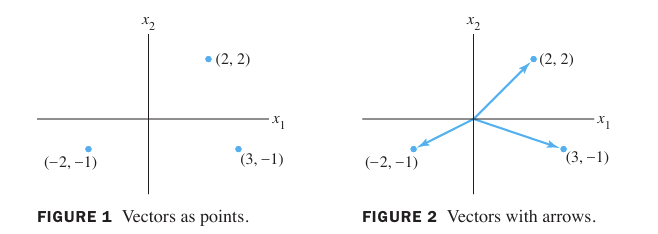
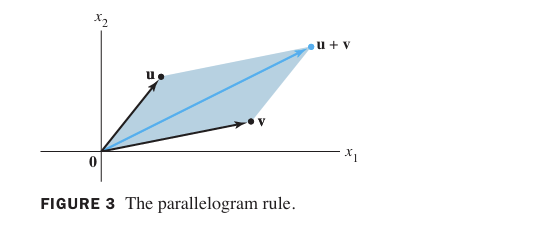
Addition follows the parallelogram rule: \(\mathbf{u}+\mathbf{v}\) is the diagonal of the parallelogram formed by \(\mathbf{u}\) and \(\mathbf{v}\).

Scalar multiplication \(c\mathbf{u}\) stretches (or shrinks) the arrow by \(|c|\), and reverses direction if \(c<0\).

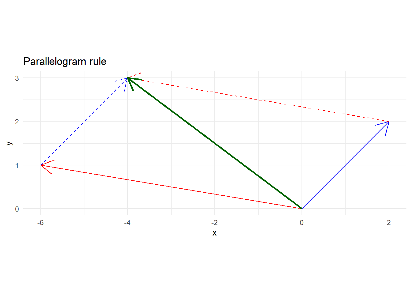
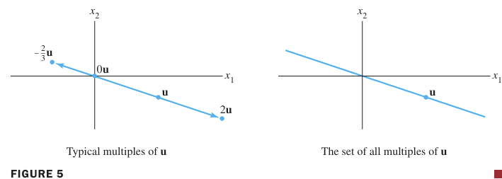
Plot showing vectors (2,2) and (-6,1) and the parallelogram — Vectors u, v and their sum (parallelogram rule illustrated in Example 2)

(This figure corresponds to textbook Figure 4.)

Example 3 (textbook). Let \(\mathbf{u} = \begin{bmatrix} 3 \\ -1 \end{bmatrix}\). The scalar multiples \(2\mathbf{u}\) and \(-\frac{2}{3}\mathbf{u}\) lie on the same line through the origin.

N.B. All scalar multiples of a nonzero vector form a line through the origin.

Vectors in \(\mathbb{R}^3\)

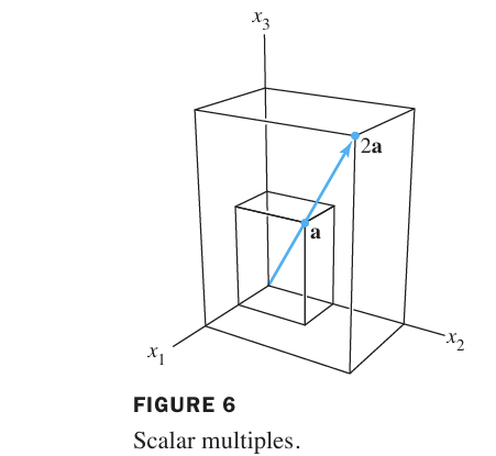
Vectors in \(\mathbb{R}^3\) are \(3\times 1\) column matrices with three entries, geometrically represented by points or arrows from the origin in \(3\)-dimensional coordinate space.

Vectors in \(\mathbb{R}^n\)

If \(n\) is a positive integer, \(\mathbb{R}^n\) consists of all column vectors with \(n\) real entries.
The zero vector \(\mathbf{0}\) has all entries zero.
Operations are defined entry‑wise, just as in \(\mathbb{R}^2\).

Algebraic properties (for \(\mathbf{u},\mathbf{v},\mathbf{w} \in \mathbb{R}^n\) and scalars \(c,d\)):

\(\mathbf{u}+\mathbf{v} = \mathbf{v}+\mathbf{u}\)
\((\mathbf{u}+\mathbf{v})+\mathbf{w} = \mathbf{u}+(\mathbf{v}+\mathbf{w})\)
\(\mathbf{u} + \mathbf{0} = \mathbf{u}\)
\(\mathbf{u} + (-\mathbf{u}) = \mathbf{0}\)
\(c(\mathbf{u}+\mathbf{v}) = c\mathbf{u} + c\mathbf{v}\)
\((c+d)\mathbf{u} = c\mathbf{u} + d\mathbf{u}\)
\(c(d\mathbf{u}) = (cd)\mathbf{u}\)
\(1\mathbf{u} = \mathbf{u}\)

Linear combinations

Given vectors \(\mathbf{v}_1, \mathbf{v}_2, \dots, \mathbf{v}_p\) in \(\mathbb{R}^n\) and scalars \(c_1, \dots, c_p\), the vector

\[\mathbf{y} = c_1 \mathbf{v}_1 + c_2 \mathbf{v}_2 + \cdots + c_p \mathbf{v}_p\]

is called a linear combination of \(\mathbf{v}_1, \dots, \mathbf{v}_p\) with weights \(c_1, \dots, c_p\).

Example 4 (textbook). Figure 8 shows linear combinations of \(\mathbf{v}_1 = \begin{bmatrix} -1 \\ 1 \end{bmatrix}\) and \(\mathbf{v}_2 = \begin{bmatrix} 2 \\ 1 \end{bmatrix}\) on a grid. Estimate the linear combinations of \(\mathbf{v}_1\) and \(\mathbf{v}_2\) that generate the vectors \(\mathbf u\) and \(\mathbf w\).

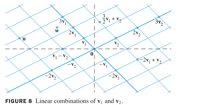
You can estimate \(\mathbf{u}\) as \(3\mathbf{v}_1 - 2\mathbf{v}_2\) and \(\mathbf{w}\) as \(\frac{5}{2}\mathbf{v}_1 - \frac{1}{2}\mathbf{v}_2\).

Comments: This expression for \(\mathbf u\) can be interpreted as instructions for traveling from the origin to \(\mathbf u\) along two straight paths. First, travel \(3\) units in the \(\mathbf{v}_1\) direction to \(3\mathbf{v}_1\),and then travel \(2\) units in the \(\mathbf{v}_2\) direction (parallel to the line through \(\mathbf{v}_2\) and \(\mathbf 0\)).

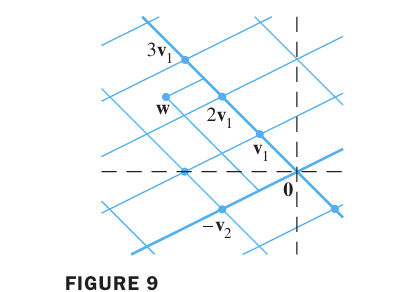
The vector \(\mathbf w\) is not on a grid line, from Figure 9, \(\mathbf w\) appears to be about halfway between two pairs of grid lines, at the vertex of a parallelogram determined by \(\frac{5}{2}\mathbf{v}_1\) and \(\frac{1}{2}\mathbf{v}_2\).

Span of a set of vectors

Definition.: If \(\mathbf{v}_1, \dots, \mathbf{v}_p\) are in \(\mathbb{R}^n\), then the set of all linear combinations of these vectors is denoted by \(\operatorname{Span}\{\mathbf{v}_1, \dots, \mathbf{v}_p\}\) and is called the subset of \(\mathbb{R}^n\) spanned (or generated) by \(\mathbf{v}_1, \dots, \mathbf{v}_p\).

Interpretations of Span:

Asking whether a vector \(\mathbf b\) is in \(\operatorname{Span}\{\mathbf{v}_1, \dots, \mathbf{v}_p\}\) amounts to asking whether the vector equation \[x_1\mathbf v_1 +x_2\mathbf v_2 + \ldots+x_p \mathbf v_p =\mathbf b\] has a solution, or, equivalently, asking whether the linear system with augmented matrix \([\mathbf v_1 \ldots\mathbf v_p \quad\mathbf b]\) has a solution.
\(\operatorname{Span}\{\mathbf{v}_1, \dots, \mathbf{v}_p\}\) contains every scalar multiple of \(\mathbf v_p\) since \(c\mathbf v_p= 0\mathbf v_1+0\mathbf v_2 + \ldots+c \mathbf v_p\)
The zero vector must be in \(\operatorname{Span}\{\mathbf{v}_1, \dots, \mathbf{v}_p\}\).

Geometric description:

For nonzero vectors \(\mathbf u\) and \(\mathbf v\) in \(\mathbb{R}^3\)

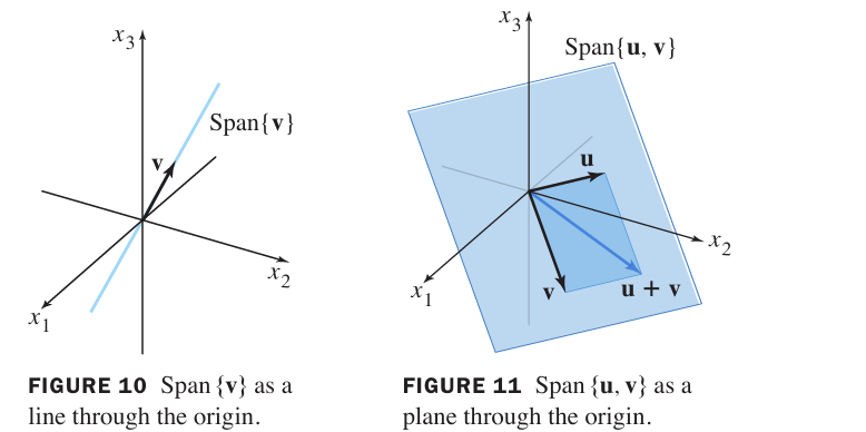
\(\operatorname{Span}\{\mathbf{v}\}\) (with \(\mathbf{v} \neq \mathbf{0}\)) is the line through the origin in the direction of \(\mathbf{v}\). (the set of all scalar multiples of \(\mathbf{v}\))
\(\operatorname{Span}\{\mathbf{u}, \mathbf{v}\}\) (with \(\mathbf{u}, \mathbf{v}\) not multiples) is a plane in \(\mathbb{R}^3\) that contains \(\mathbf u\), \(\mathbf v\) and the origin. (\(\operatorname{Span}\{\mathbf{u}, \mathbf{v}\}\) contains line in \(\mathbb{R}^3\) through \(\mathbf u\) and the \(\mathbf 0\) and line through \(\mathbf u\) and \(\mathbf 0\).)

Example 5 (textbook). Let \(\mathbf{a}_1 = \begin{bmatrix} 1 \\ -2 \\ -5 \end{bmatrix}\), \(\mathbf{a}_2 = \begin{bmatrix} 2 \\ 5 \\ 6 \end{bmatrix}\), \(\mathbf{b} = \begin{bmatrix} 7 \\ 4 \\ -3 \end{bmatrix}\). Is \(\mathbf{b}\) a linear combination of \(\mathbf{a}_1\) and \(\mathbf{a}_2\)?

We ask: does there exist \(x_1, x_2\) such that

\[x_1 \mathbf{a}_1 + x_2 \mathbf{a}_2 = \mathbf{b} \quad\text{?}\]

This is the vector equation

\[x_1 \begin{bmatrix} 1 \\ -2 \\ -5 \end{bmatrix} + x_2 \begin{bmatrix} 2 \\ 5 \\ 6 \end{bmatrix} = \begin{bmatrix} 7 \\ 4 \\ -3 \end{bmatrix}.\]

It corresponds to the linear system with augmented matrix \([\,\mathbf{a}_1\;\mathbf{a}_2\;\mathbf{b}\,]\):

\[\left[\begin{array}{cc|c} 1 & 2 & 7 \\ -2 & 5 & 4 \\ -5 & 6 & -3 \end{array}\right].\]

Row reduction yields (details as in textbook):

\[\left[\begin{array}{cc|c} 1 & 0 & 3 \\ 0 & 1 & 2 \\ 0 & 0 & 0 \end{array}\right].\]

Thus \(x_1 = 3\), \(x_2 = 2\), and \(\mathbf{b} = 3\mathbf{a}_1 + 2\mathbf{a}_2\). So \(\mathbf{b}\) is in \(\operatorname{Span}\{\mathbf{a}_1,\mathbf{a}_2\}\).

N.B. 1. A vector equation \[x_1\mathbf a_1 +x_2\mathbf a_2 + \ldots+x_n \mathbf a_n =\mathbf b\] has the same solution set as the linear system whose augmented matrix is \[[\mathbf a_1 \quad \mathbf a_2 \ldots\mathbf a_n \quad\mathbf b]\] N.B. 2. \(\mathbf b\) can be generated by a linear combination of \(\mathbf a_1, \mathbf a_2 \ldots\mathbf a_n\) if and only if there exists a solution to the linear system corresponding to the augmented matrix. (Interpretations of Span)

Example 6 (textbook). Let \(\mathbf{a}_1 = \begin{bmatrix} 1 \\ -2 \\ 3 \end{bmatrix}\), \(\mathbf{a}_2 = \begin{bmatrix} 5 \\ -13 \\ -3 \end{bmatrix}\), \(\mathbf{b} = \begin{bmatrix} -3 \\ 8 \\ 1 \end{bmatrix}\)

Span of vectors \(\mathbf a_1, \mathbf a_2\) in \(\mathbb{R}^3\) forms a plane; we check if a vector \(\mathbf b\) lies in that plane by solving a linear system. If the system is inconsistent, the vector is not in the span.
Still, We ask: does there exist \(x_1, x_2\) such that

\[x_1 \mathbf{a}_1 + x_2 \mathbf{a}_2 = \mathbf{b} \quad\text{?}\]

The linear system with augmented matrix \([\,\mathbf{a}_1\;\mathbf{a}_2\;\mathbf{b}\,]\):

\[\left[\begin{array}{cc|c} 1 & 5 & -3 \\ -2 & -13 & 8 \\ 3 & -3 & 1 \end{array}\right].\]

Row reduction yields (details as in textbook):

\[\left[\begin{array}{cc|c} 1 & 5 & -3 \\ 0 & -3 & 2 \\ 0 & 0 & -2 \end{array}\right].\]

The system has no solution, therefore vector \(\mathbf b\) is not in \(\operatorname{Span}\{\mathbf a_1, \mathbf a_2\}\).

Section 1.4 The Matrix Equation \(A\mathbf{x} = \mathbf{b}\)

Learning Objectives

After this lecture you will be able to:

Express a system of linear equations as a vector equation and as a matrix equation \(A\mathbf{x} = \mathbf{b}\).
Compute the product of a matrix and a vector using the column method and the row‑vector rule.
State and apply the equivalence of the linear system, vector equation, and matrix equation.
Use Theorem 4 to decide when the columns of a matrix span \(\mathbb{R}^m\).

Multiplication of a matrix and a vector

Definition: If \(A\) is an \(m \times n\) matrix with columns \(\mathbf{a}_1, \dots, \mathbf{a}_n\), and \(\mathbf{x} \in \mathbb{R}^n\), then the product \(A\mathbf{x}\) is the linear combination of the columns of \(A\) with weights given by the entries of \(\mathbf{x}\):

\[A\mathbf{x} = \begin{bmatrix} \mathbf{a}_1 & \mathbf{a}_2 & \cdots & \mathbf{a}_n \end{bmatrix} \begin{bmatrix} x_1 \\ x_2 \\ \vdots \\ x_n \end{bmatrix} = x_1 \mathbf{a}_1 + x_2 \mathbf{a}_2 + \cdots + x_n \mathbf{a}_n.\]

N.B. \(A\mathbf{x}\) is defined only if the number of columns of \(A\) equals the number of entries in \(\mathbf{x}\).

Example 1 (textbook).

\[\begin{aligned} \text{(a)}\quad \begin{bmatrix} 1 & 2 & -1 \\ 0 & -5 & 3 \end{bmatrix} \begin{bmatrix} 4 \\ 3 \\ 7 \end{bmatrix} &= 4\begin{bmatrix} 1 \\ 0 \end{bmatrix} + 3\begin{bmatrix} 2 \\ -5 \end{bmatrix} + 7\begin{bmatrix} -1 \\ 3 \end{bmatrix} \\ &= \begin{bmatrix} 4 \\ 0 \end{bmatrix} + \begin{bmatrix} 6 \\ -15 \end{bmatrix} + \begin{bmatrix} -7 \\ 21 \end{bmatrix} = \begin{bmatrix} 3 \\ 6 \end{bmatrix}. \end{aligned}\]

(b)

Example 2 (textbook). For \(\mathbf v_1, \mathbf v_2, \mathbf v_3\) in \(\mathbb R^m\), write the linear combination \(3\mathbf v_1 -5 \mathbf v_2 +7 \mathbf v_3\) as a matrix times a vector.

Computation of \(A\mathbf{x}\)

Row-Vector Rule for Computing \(A\mathbf{x}\)

If \(A\mathbf{x}\) is defined, the \(i\)th entry of \(A\mathbf{x}\) is the sum of the products of the entries in row \(i\) of \(A\) with the corresponding entries of \(\mathbf{x}\). This is convenient for hand calculations.

Example 4 (textbook). Compute \(A\mathbf{x}\) with \(A = \begin{bmatrix} 2 & 3 & 4 \\ -1 & 5 & -3 \\ 6 & -2 & 8 \end{bmatrix}\), \(\mathbf{x} = \begin{bmatrix} x_1 \\ x_2 \\ x_3 \end{bmatrix}\).

\[A\mathbf{x} = \begin{bmatrix} 2x_1 + 3x_2 + 4x_3 \\ -x_1 + 5x_2 - 3x_3 \\ 6x_1 - 2x_2 + 8x_3 \end{bmatrix}.\]

N.B. The equation in the form \(A\mathbf{x} = \mathbf{b}\) is called a matrix equation.

Theorem 3

Theorem 3.

If \(A\) is an \(m \times n\) matrix with columns \(\mathbf{a}_1, \dots, \mathbf{a}_n\), and if \(\mathbf b\) is in \(\mathbb R^m\), then,

the matrix equation \(A\mathbf{x} = \mathbf{b}\), the vector equation \(x_1\mathbf{a}_1 + \cdots + x_n\mathbf{a}_n = \mathbf{b}\), and the linear system with augmented matrix \([\,\mathbf{a}_1 \; \dots \; \mathbf{a}_n \; \mathbf{b}\,]\) all have the same solution set.

Interpretations:

Solving \(A\mathbf{x} = \mathbf{b}\) means finding all linear combinations of the columns of \(A\) that produce \(\mathbf{b}\).
Existence of a solution is equivalent to \(\mathbf{b}\) being in \(\operatorname{Span}\{\mathbf{a}_1,\dots,\mathbf{a}_n\}\).
When you construct a mathematical model of a problem in real life, you are free to choose whichever viewpoint is most natural. Then you may switch from one formulation of a problem to another whenever it is convenient – the system of equations are all solved by row reducing the augmented matrix. (Other methods of solution will be discussed later.)

Existence of solutions

The equation \(A\mathbf{x} = \mathbf{b}\) has a solution if and only if \(\mathbf{b}\) is a linear combination of the columns of \(A\).

N.B. Existence of a solution is equivalent to \(\mathbf{b}\) being in \(\operatorname{Span}\{\mathbf{a}_1,\dots,\mathbf{a}_n\}\).

A general question: Is equation \(A\mathbf{x} = \mathbf{b}\) consistent for all possible \(\mathbf{b}\)?

Example 3 (textbook). Let

\[A = \begin{bmatrix} 1 & 3 & 4 \\ -4 & 2 & -6 \\ -3 & -2 & -7 \end{bmatrix},\quad \mathbf{b} = \begin{bmatrix} b_1 \\ b_2 \\ b_3 \end{bmatrix}.\]

Is the equation \(A\mathbf{x} = \mathbf{b}\) consistent for all \(\mathbf{b}\)?
Row reduce the augmented matrix:

\[\left[\begin{array}{ccc|c} 1 & 3 & 4 & b_1 \\ -4 & 2 & -6 & b_2 \\ -3 & -2 & -7 & b_3 \end{array}\right] \sim \left[\begin{array}{ccc|c} 1 & 3 & 4 & b_1 \\ 0 & 14 & 10 & b_2+4b_1 \\ 0 & 7 & 5 & b_3+3b_1 \end{array}\right] \sim \left[\begin{array}{ccc|c} 1 & 3 & 4 & b_1 \\ 0 & 14 & 10 & b_2+4b_1 \\ 0 & 0 & 0 & b_3+3b_1-\frac{1}{2}(b_2+4b_1) \end{array}\right].\]

The reduced matrix provides a description of all \(\mathbf{b}\) for which the equation \(A\mathbf{x} = \mathbf{b}\) is consistent:The entries in \(\mathbf{b}\) must satisfy \[b_3+3b_1-\frac{1}{2}(b_2+4b_1) = 0\] So \(A\mathbf{x} = \mathbf{b}\) is not consistent for all \(\mathbf{b}\).

N.B. The system is consistent only if \(b_3+3b_1-\frac{1}{2}(b_2+4b_1) = 0\). This is the equation of a plane through the origin in \(\mathbb R^3\).

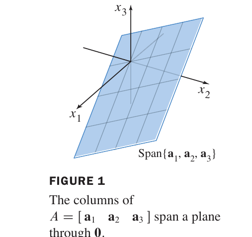
(The plane is the set of all linear combinations of the three columns of \(A\).)

Theorem 4

Theorem 4.

Let \(A\) be an \(m \times n\) matrix. The following statements are equivalent:

For each \(\mathbf{b} \in \mathbb{R}^m\), the equation \(A\mathbf{x} = \mathbf{b}\) has a solution.
Each \(\mathbf{b} \in \mathbb{R}^m\) is a linear combination of the columns of \(A\).
The columns of \(A\) span \(\mathbb{R}^m\).
\(A\) has a pivot position in every row.

Interpretations: e.g., The sentence “The columns of \(A\) span \(\mathbb{R}^m\)” means that every \(\mathbf{b} \in \mathbb{R}^m\) is a linear combination of the columns of \(A\).

N.B. This is a powerful result: to check if the columns span the whole space, just reduce \(A\) to echelon form and see if every row contains a pivot. (Theorem 4 (d) implies \(m\leq n\))

Example. A \(3 \times 2\) matrix cannot have a pivot in every row (only 2 columns), so its columns cannot span \(\mathbb{R}^3\). Therefore, a set of two vectors in \(\mathbb{R}^3\) cannot span \(\mathbb{R}^3\).

N.B. Theorem 4 is about a coefficient matrix, not an augmented matrix. If an augmented matrix \([A \quad\mathbf b]\) has a pivot position in every row,then the equation \(A\mathbf{x} = \mathbf{b}\) may or may not be consistent.

Theorem 5 - Properties of \(A\mathbf{x}\)

Theorem 5.

If \(A\) is \(m \times n\), \(\mathbf{u}, \mathbf{v} \in \mathbb{R}^n\), and \(c\) is a scalar, then

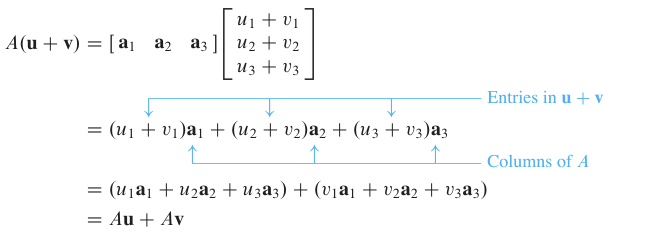
\(A(\mathbf{u} + \mathbf{v}) = A\mathbf{u} + A\mathbf{v}\)
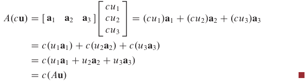
\(A(c\mathbf{u}) = c(A\mathbf{u})\)

These properties make the transformation \(\mathbf{x} \mapsto A\mathbf{x}\) a linear transformation (a preview of Sections 1.8-1.9).

Proof of Theorem 5 is optional.

Practice problems (in-class)

Compute \(2\mathbf{u} - 3\mathbf{v}\) for \(\mathbf{u} = \begin{bmatrix} 4 \\ -2 \end{bmatrix}\), \(\mathbf{v} = \begin{bmatrix} -1 \\ 3 \end{bmatrix}\). Draw the result on a graph.
Determine if \(\mathbf{b} = \begin{bmatrix} 4 \\ 1 \\ -3 \end{bmatrix}\) is a linear combination of \(\mathbf{a}_1 = \begin{bmatrix} 1 \\ 2 \\ -1 \end{bmatrix}\) and \(\mathbf{a}_2 = \begin{bmatrix} -2 \\ 3 \\ 1 \end{bmatrix}\).
Set up the vector equation and solve.
Let \(A = \begin{bmatrix} 2 & 0 & 1 \\ 1 & -1 & 2 \end{bmatrix}\), \(\mathbf{x} = \begin{bmatrix} 3 \\ -1 \\ 2 \end{bmatrix}\). Compute \(A\mathbf{x}\) using both the definition (column combination) and the row-vector rule. Verify they agree.
Does the equation \(A\mathbf{x} = \mathbf{b}\) have a solution for every \(\mathbf{b} \in \mathbb{R}^3\) if

\[A = \begin{bmatrix} 1 & 3 & -2 \\ 0 & 1 & 4 \\ 2 & 5 & -8 \end{bmatrix}\ ?\]
Write the system

\[\begin{aligned} 2x_1 - x_2 + 3x_3 &= 5 \\ x_1 + 4x_2 &= 7 \end{aligned}\]

as a vector equation and as a matrix equation \(A\mathbf{x} = \mathbf{b}\).

(Solutions follow at the end.)

R supplement

We can work with vectors and matrices directly.

# Define vectors in R^2
u <- c(1, -2)
v <- c(2, -5)
4*u

[1]  4 -8

(-3)*v

[1] -6 15

4*u + (-3)*v

[1] -2  7

# Check if b is a linear combination of a1, a2 
A <- matrix(c(1, -2, -5,   # a1
              2,  5,  6),  # a2
            nrow=3, byrow=FALSE)
b <- c(7, 4, -3)
aug <- cbind(A, b)
# Use qr.solve for non-square (overdetermined) consistent systems
x <- qr.solve(A, b)
x   # should be 3, 2

[1] 3 2

The output gives \(x_1=3\), \(x_2=2\), confirming \(\mathbf{b}\) is a combination.

Solutions to practice problems

\(2\mathbf{u} - 3\mathbf{v} = 2\begin{bmatrix}4\\-2\end{bmatrix} - 3\begin{bmatrix}-1\\3\end{bmatrix} = \begin{bmatrix}8\\-4\end{bmatrix} - \begin{bmatrix}-3\\9\end{bmatrix} = \begin{bmatrix}11\\-13\end{bmatrix}\).
The vector points from the origin to \((11,-13)\).
Vector equation: \(x_1 \begin{bmatrix}1\\2\\-1\end{bmatrix} + x_2 \begin{bmatrix}-2\\3\\1\end{bmatrix} = \begin{bmatrix}4\\1\\-3\end{bmatrix}\).
Augmented matrix:

\[\left[\begin{array}{cc|c} 1 & -2 & 4 \\ 2 & 3 & 1 \\ -1 & 1 & -3 \end{array}\right] \sim \left[\begin{array}{cc|c} 1 & 0 & 2 \\ 0 & 1 & -1 \\ 0 & 0 & 0 \end{array}\right].\] So \(x_1=2\), \(x_2=-1\).
Using columns:

\[A\mathbf{x} = 3\begin{bmatrix}2\\1\end{bmatrix} + (-1)\begin{bmatrix}0\\-1\end{bmatrix} + 2\begin{bmatrix}1\\2\end{bmatrix} = \begin{bmatrix}6\\3\end{bmatrix} + \begin{bmatrix}0\\1\end{bmatrix} + \begin{bmatrix}2\\4\end{bmatrix} = \begin{bmatrix}8\\8\end{bmatrix}.\]
Row reduce \(A\): the echelon form has a row of zeros, so \(A\) does not have a pivot in every row. By Theorem 4, the equation does not have a solution for every \(\mathbf b\in\mathbb{R}^3\).
Vector equation:

\[x_1 \begin{bmatrix} 2 \\ 1 \end{bmatrix} + x_2 \begin{bmatrix} -1 \\ 4 \end{bmatrix} + x_3 \begin{bmatrix} 3 \\ 0 \end{bmatrix} = \begin{bmatrix} 5 \\ 7 \end{bmatrix}.\] Matrix equation: \[\begin{bmatrix} 2 & -1 & 3 \\ 1 & 4 & 0 \end{bmatrix} \begin{bmatrix} x_1 \\ x_2 \\ x_3 \end{bmatrix} = \begin{bmatrix} 5 \\ 7 \end{bmatrix}.\]

Summary

Vectors are ordered lists of numbers; operations act entry-wise.
A linear combination of vectors is the fundamental building block.
The span of a set describes all vectors reachable by linear combinations.
The matrix product \(A\mathbf{x}\) is exactly the linear combination of the columns of \(A\) with weights \(x_j\).
Solving \(A\mathbf{x} = \mathbf{b}\) is the same as asking whether \(\mathbf{b}\) is in the span of the columns of \(A\).
A matrix \(A\) has the property that \(A\mathbf{x} = \mathbf{b}\) is solvable for every \(\mathbf{b}\) if and only if \(A\) has a pivot in every row.
Next time we study homogeneous systems and linear independence.

Section 1.5 Solution Sets of Linear Systems

Learning Objectives

After this lecture you will be able to:

Determine if a homogeneous linear system has nontrivial solutions.
Describe the solution set of a homogeneous system in parametric vector form.
Understand the relationship between the solution sets of \(A\mathbf{x} = \mathbf{0}\) and \(A\mathbf{x} = \mathbf{b}\).
Write the general solution of a consistent non‑homogeneous system as a particular solution plus the solution of the associated homogeneous system.

Homogeneous Linear Systems

A system of linear equations is homogeneous if it can be written as \(A\mathbf{x} = \mathbf{0}\), where \(A\) is an \(m \times n\) matrix and \(\mathbf{0}\) is the zero vector in \(\mathbb{R}^m\).
Such a system always has at least one solution: \(\mathbf{x} = \mathbf{0}\) (the trivial solution).
The important question is whether there exist nontrivial solutions (nonzero vectors \(\mathbf{x}\) satisfying \(A\mathbf{x} = \mathbf{0}\)).

Fact:: The homogeneous equation \(A\mathbf{x} = \mathbf{0}\) has a nontrivial solution if and only if the equation has at least one free variable.
(This follows from the Existence and Uniqueness Theorem of Section 1.2.)

Example 1 (textbook): Determine if the system has a nontrivial solution, then describe the solution set.

\[\begin{aligned} 3x_1 + 5x_2 - 4x_3 &= 0 \\ -3x_1 -2x_2 +4x_3 &= 0 \\ 6x_1 +x_2 -8x_3 &= 0 \end{aligned}\]

Solution. Write the augmented matrix \([A \; \mathbf{0}]\) and row reduce to echelon form:

\[\left[\begin{array}{ccc|c} 3 & 5 & -4 & 0 \\ -3 & -2 & 4 & 0 \\ 6 & 1 & -8 & 0 \end{array}\right] \sim \left[\begin{array}{ccc|c} 3 & 5 & -4 & 0 \\ 0 & 3 & 0 & 0 \\ 0 & -9 & 0 & 0 \end{array}\right] \sim \left[\begin{array}{ccc|c} 3 & 5 & -4 & 0 \\ 0 & 3 & 0 & 0 \\ 0 & 0 & 0 & 0 \end{array}\right].\]

There is a free variable (\(x_3\)), so nontrivial solutions exist.
Continue to reduced echelon form:

\[\left[\begin{array}{ccc|c} 1 & 0 & -\frac{4}{3} & 0 \\ 0 & 1 & 0 & 0 \\ 0 & 0 & 0 & 0 \end{array}\right].\]

The corresponding system: \(x_1 -\frac{4}{3}x_3 = 0\), \(x_2 = 0\).
Basic variables: \(x_1\), \(x_2\); free variable: \(x_3\). Solve for basic variables:

\[x_1 = \frac{4}{3}x_3,\quad x_2 =0,\quad x_3 \text{ free}.\]

In parametric vector form, the general solution is

\[\mathbf{x} = \begin{bmatrix} x_1 \\ x_2 \\ x_3 \end{bmatrix} = \begin{bmatrix}\frac{4}{3}x_3\\ 0 \\ x_3 \end{bmatrix} = x_3 \begin{bmatrix} \frac{4}{3} \\ 0 \\ 1 \end{bmatrix}.\]

Letting \(t = x_3\), the solution set is \(\{ t\mathbf{v} \mid t \in \mathbb{R}\}\) with \(\mathbf{v} = \begin{bmatrix} \frac{4}{3} \\ 0 \\ 1 \end{bmatrix}\).
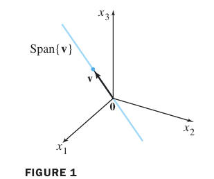
Geometrically, this is a line through the origin in \(\mathbb{R}^3\).

Example 2 (textbook): A single homogeneous equation

Example 2: Describe all solutions to the homogeneous “system” \(10x_1 - 3x_2 - 2x_3 = 0\).

Solution: There is no need for matrix notation.

The general solution is obtained by solving for the basic variable \(x_1\) in terms of the free variables \(x_2\), \(x_3\):

\[x_1 = 0.3x_2 + 0.2x_3.\]

In vector form:

\[\mathbf{x} = \begin{bmatrix} x_1 \\ x_2 \\ x_3 \end{bmatrix} = \begin{bmatrix} 0.3x_2 + 0.2x_3 \\ x_2 \\ x_3 \end{bmatrix} = x_2 \begin{bmatrix} 0.3 \\ 1 \\ 0 \end{bmatrix} + x_3 \begin{bmatrix} 0.2 \\ 0 \\ 1 \end{bmatrix}.\]

Thus the solution set is \(\operatorname{Span}\{\mathbf{u}, \mathbf{v}\}\) with \(\mathbf{u} = \begin{bmatrix} 0.3 \\ 1 \\ 0 \end{bmatrix}\), \(\mathbf{v} = \begin{bmatrix} 0.2 \\ 0 \\ 1 \end{bmatrix}\).
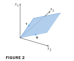
Since \(\mathbf{u}\) and \(\mathbf{v}\) are not multiples of each other, the solution set is a plane through the origin in \(\mathbb{R}^3\).

In general, the solution set of a homogeneous equation \(A\mathbf x=\mathbf 0\) can always be expressed explicitly as \(\operatorname{Span}\{\mathbf{v}_1,\ldots, \mathbf{v}_p\}\) for suitable vectors \(\mathbf{v}_1,\ldots, \mathbf{v}_p\).

Example 1&2 illustrate the fact for the special case in \(\mathbb{R}^3\)

If the only solution is the zero vector, then the solution set is \(\operatorname{Span}\{\mathbf 0\}\).
If the equation \(A\mathbf x=\mathbf 0\) has only one free variable, the solution set is a line through the origin ( Figure 1).
If there are two free variables, the solution set is a plane through the origin (Figure 2).
If there are three free variables, the solution set is the whole space (\(\mathbb{R}^3=\operatorname{Span}\{\mathbf e_1,\mathbf e_2, \mathbf e_3\}\)).

Parametric Vector Form

For a consistent homogeneous or non‑homogeneous system, expressing the solution set with vectors (as above) is called parametric vector form, such as \[\mathbf x= s\mathbf u+t\mathbf v\quad (s,t \text{ in } \mathbb R)\]
In Example 1, \(\mathbf x = x_3 \mathbf v\) with \(x_3\) free , or alternatively \(\mathbf x=t\mathbf v\) with \(t\) in \(\mathbb R\).

It shows the solution set explicitly as a linear combination (span) of vectors, plus possibly a particular solution.

Comments: When a nonhomogeneous linear system has many solutions, the general solution can be written in parametric vector form as one vector (a particular solution) plus an arbitrary linear combination of vectors that satisfy the corresponding homogeneous system.

Theorem 6 - Solutions of Non‑homogeneous Systems

Consider a consistent system \(A\mathbf{x} = \mathbf{b}\). Let \(\mathbf{p}\) be a particular solution (one specific solution).
Then every solution of \(A\mathbf{x} = \mathbf{b}\) can be written as

\[\mathbf{x} = \mathbf{p} + \mathbf{v}_h,\]

where \(\mathbf{v}_h\) is some solution of the homogeneous equation \(A\mathbf{x} = \mathbf{0}\).

Theorem 6.: Suppose equation \(A\mathbf{x} = \mathbf{b}\) is consistent for some given \(\mathbf b\) and let \(\mathbf{p}\) be a solution. Then the solution set of \(A\mathbf{x} = \mathbf{b}\) is the set of all vectors of the form \(\mathbf w=\mathbf{p} + \mathbf{v}_h\), ,where \(\mathbf{v}_h\) is any solution of the homogeneous equation \(A\mathbf{x} = \mathbf 0\), i.e., \[\{\mathbf{p} + \mathbf{v}_h \mid \mathbf{v}_h \in \text{solution set of } A\mathbf{x} = \mathbf 0 \}\]

Geometrically, the solution set of \(A\mathbf{x} = \mathbf{b}\) is the translation of the solution set of \(A\mathbf{x} = \mathbf{0}\) by the vector \(\mathbf{p}\).

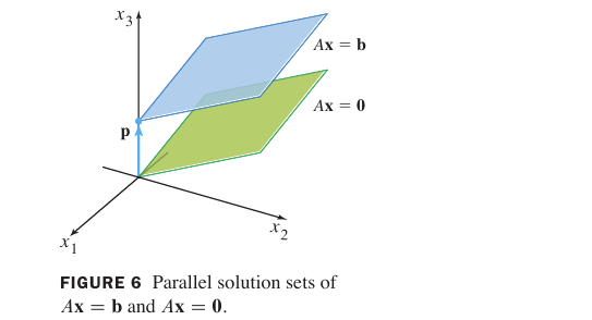
N.B. Theorem 6 and Figure 6 apply only to an equation \(A\mathbf{x} = \mathbf{b}\) that has at least one nonzero solution \(\mathbf{p}\). When \(A\mathbf{x} = \mathbf{b}\) has no solution, the solution set is empty.

Example 3 (textbook). Describe all solutions of \(A\mathbf{x} = \mathbf{b}\) where \(A\) is the coefficient matrix from Example 1 and \(\mathbf{b} = \begin{bmatrix} 7 \\ -1 \\ 4 \end{bmatrix}\).

Row reduction of \([A \; \mathbf{b}]\) yields (after the same steps) the reduced echelon form

\[\left[\begin{array}{ccc|c} 1 & 0 & -\frac{4}{3} & -1 \\ 0 & 1 & 0 & 2 \\ 0 & 0 & 0 & 0 \end{array}\right].\]

Thus \(x_1 = -1 +\frac{4}{3}x_3\), \(x_2 = 2\), \(x_3\) free. In parametric vector form, the general solution is:

\[\mathbf{x} = \begin{bmatrix} -1 \\ 2 \\ 0 \end{bmatrix} + x_3 \begin{bmatrix} \frac{4}{3} \\ 0 \\ 1 \end{bmatrix}.\]

Here \(\mathbf{p} = \begin{bmatrix} -1 \\ 2 \\ 0 \end{bmatrix}\) is a particular solution, and \(\mathbf{v} = \begin{bmatrix} \frac{4}{3} \\ 0 \\ 1 \end{bmatrix}\) generates the homogeneous solution set.

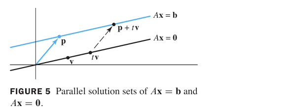
N.B. Using general parameter \(t\), \[\mathbf{x} =\mathbf{p}+ t\mathbf{v}\quad (t \text{ in } \mathbb R)\]

Considering the vector addition as a translation, the solution set is a line through \(\mathbf{p}\) parallel to \(\mathbf{v}\).

Section 1.7 Linear Independence

Learning Objectives

After this lecture you will be able to:

Define linear independence of a set of vectors.
Determine by inspection or by solving \(A\mathbf{x} = \mathbf{0}\) whether a set of vectors is linearly independent.
Apply theorems about linear dependence involving many vectors, relations among them, and the presence of the zero vector.

An indexed set of vectors \(\{\mathbf{v}_1, \dots, \mathbf{v}_p\}\) in \(\mathbb{R}^n\) is linearly independent if the vector equation

\[x_1 \mathbf{v}_1 + x_2 \mathbf{v}_2 + \cdots + x_p \mathbf{v}_p = \mathbf{0}\]

has only the trivial solution \(x_1 = \cdots = x_p = 0\).
The set \(\{\mathbf{v}_1, \dots, \mathbf{v}_p\}\) is linearly dependent if there exist weights \(c_1, \dots, c_p\), not all zero, such that

\[c_1 \mathbf{v}_1 + c_2 \mathbf{v}_2 + \cdots + c_p \mathbf{v}_p = \mathbf{0}.\]

Such an equation is called a linear dependence relation among the vectors \(\mathbf{v}_1, \dots, \mathbf{v}_p\).

For brevity, we may say that \(\mathbf{v}_1, \dots, \mathbf{v}_p\) are linearly dependent when \(\{\mathbf{v}_1, \dots, \mathbf{v}_p\}\) is a linearly dependent set.

Example 1 (textbook): Linear dependence in \(\mathbb{R}^3\)

Let \(\mathbf{v}_1 = \begin{bmatrix} 1 \\ 2 \\ 3 \end{bmatrix}\), \(\mathbf{v}_2 = \begin{bmatrix} 4 \\ 5 \\ 6 \end{bmatrix}\), \(\mathbf{v}_3 = \begin{bmatrix} 2 \\ 1 \\ 0 \end{bmatrix}\).
(a) Determine if \(\{\mathbf{v}_1, \mathbf{v}_2, \mathbf{v}_3\}\) is linearly independent.
(b) If possible, find a linear dependence relation.

Solution. Solve \(x_1\mathbf{v}_1 + x_2\mathbf{v}_2 + x_3\mathbf{v}_3 = \mathbf{0}\). Augmented matrix:

\[\left[\begin{array}{ccc|c} 1 & 4 & 2 & 0 \\ 2 & 5 & 1 & 0 \\ 3 & 6 & 0 & 0 \end{array}\right] \sim \left[\begin{array}{ccc|c} 1 & 4 & 2 & 0 \\ 0 & -3 & -3 & 0 \\ 0 & -6 & -6 & 0 \end{array}\right] \sim \left[\begin{array}{ccc|c} 1 & 4 & 2 & 0 \\ 0 & 1 & 1 & 0 \\ 0 & 0 & 0 & 0 \end{array}\right].\]

There is a free variable (\(x_3\)), so each nonzero value of \(x_3\) determines a nontrivial solution. Thus, nontrivial solutions exist: the set is linearly dependent.
To find a dependence relation, continue to reduced echelon:

\[\left[\begin{array}{ccc|c} 1 & 0 & -2 & 0 \\ 0 & 1 & 1 & 0 \\ 0 & 0 & 0 & 0 \end{array}\right] \Longrightarrow \begin{aligned} x_1 &= 2x_3 \\ x_2 &= -x_3 \\ x_3 &\text{ free} \end{aligned}\] Choose any nonzero value for \(x_3\), for example:

Choose \(x_3 = 1\), then \(x_1 = 2\), \(x_2 = -1\), yielding

\[2\mathbf{v}_1 - \mathbf{v}_2 + \mathbf{v}_3 = \mathbf{0},\]

a linear dependence relation.

Linear Independence of Matrix Columns

If we place the vectors as columns of a matrix \(A = [\mathbf{a}_1 \cdots \mathbf{a}_n]\), then

\[A\mathbf{x} = \mathbf{0} \quad\Longleftrightarrow\quad x_1\mathbf{a}_1 + \cdots + x_n\mathbf{a}_n = \mathbf{0}.\]

Thus we have the following important fact:: The columns of a matrix \(A\) are linearly independent if and only if the equation \(A\mathbf{x} = \mathbf{0}\) has only the trivial solution.

Example 2 (textbook). Determine if the columns of \(A = \begin{bmatrix} 0 & 1 & 4 \\ 1 & 2 & -1 \\ 5 & 8 & 0 \end{bmatrix}\) are linearly independent.

Row reduce \(A\) (or alternatively row reduce the augmented matrix):

\[\begin{bmatrix} 0 & 1 & 4 \\ 1 & 2 & -1 \\ 5 & 8 & 0 \end{bmatrix} \sim \begin{bmatrix} 1 & 2 & -1 \\ 0 & 1 & 4 \\ 0 & -2 & 5 \end{bmatrix} \sim \begin{bmatrix} 1 & 2 & -1 \\ 0 & 1 & 4 \\ 0 & 0 & 13 \end{bmatrix}.\]

There are three basic variables and no free variables. All three columns are pivot columns, so \(A\mathbf{x} = \mathbf{0}\) has only the trivial solution. The columns are linearly independent.

Sets of One or Two Vectors

A set containing a single vector \(\mathbf{v}\) is linearly independent iff \(\mathbf{v} \neq \mathbf{0}\). (\(x_1\mathbf v=\mathbf 0\) has only the trivial solution when \(\mathbf{v} \neq \mathbf{0}\))
A set of two vectors \(\{\mathbf{v}_1, \mathbf{v}_2\}\) is linearly dependent iff at least one vector is a scalar multiple of the other.
(Geometrically, they lie on the same line through the origin.)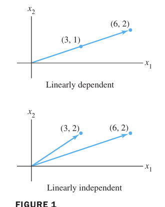

(Figure 1: The set \(\{\mathbf{v}_1, \mathbf{v}_2\}\) is linearly independent if and only if neither of the vectors is a multiple of the other.)

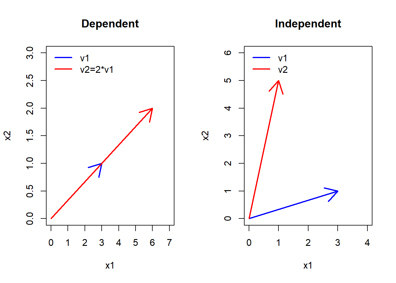
Example 3 (textbook).
(a) \(\begin{bmatrix} 3 \\ 1 \end{bmatrix}\) and \(\begin{bmatrix} 6 \\ 2 \end{bmatrix}\) are dependent (second is \(2\times\) first).
(b) \(\begin{bmatrix} 3 \\ 1 \end{bmatrix}\) and \(\begin{bmatrix} 1 \\ 5 \end{bmatrix}\) are independent (neither is a multiple of the other).

Plot of two sets of vectors showing dependence vs independence — Left: linearly dependent (on same line); Right: linearly independent

Sets of Two or More Vectors

Theorem 7

Theorem 7. Characterization of Linearly Dependent Sets: An indexed set \(S = \{\mathbf{v}_1, \dots, \mathbf{v}_p\}\) of two or more vectors is linearly dependent iff at least one of the vectors in \(S\) is a linear combination of the others. In fact, if \(S\) is linearly dependent and \(\mathbf{v}_1 \neq \mathbf{0}\), then some \(\mathbf{v}_j\) (with \(j > 1\)) is a linear combination of the preceding vectors \(\mathbf{v}_1, \dots, \mathbf{v}_{j-1}\).

N.B. A direct consequence of theorem 7: any set containing a dependent subset is dependent.

N.B. Not every vector in a dependent set must be a combination of the others; only at least one.

Warning: Theorem 7 does not say that every vector in a linearly dependent set is a linear combination of the preceding vectors. A vector in a linearly dependent set may fail to be a linear combination of the other vectors.

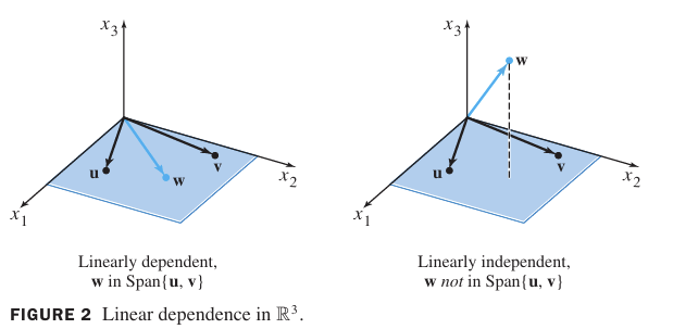
Example 4 (textbook). Let \(\mathbf{u} = \begin{bmatrix} 3 \\ 1 \\ 0 \end{bmatrix}\) and \(\mathbf{v} = \begin{bmatrix} 1 \\ 6 \\ 0 \end{bmatrix}\). Describe \(\operatorname{Span}\{\mathbf{u},\mathbf{v}\}\) and explain why a vector \(\mathbf{w}\) is in \(\operatorname{Span}\{\mathbf{u},\mathbf{v}\}\) iff \(\{\mathbf{u},\mathbf{v},\mathbf{w}\}\) is linearly dependent.

\(\mathbf{u}\) and \(\mathbf{v}\) are independent (not multiples), so \(\operatorname{Span}\{\mathbf{u},\mathbf{v}\}\) is a plane through the origin in \(\mathbb R^3\) (the \(x_1x_2\)-plane with \(x_3=0\)).
If \(\mathbf{w} \in \operatorname{Span}\{\mathbf{u},\mathbf{v}\}\), then \(\mathbf{w} = c\mathbf{u} + d\mathbf{v}\), so \(c\mathbf{u}+d\mathbf{v} - \mathbf{w} = \mathbf{0}\), a nontrivial combination (weight on \(\mathbf{w}\) is \(-1\)). Thus the set is dependent. Conversely, if dependent, by Theorem 7 one vector is a combination of the others. Since \(\mathbf{u},\mathbf{v}\) are independent, that vector must be \(\mathbf{w}\), so \(\mathbf{w} \in \operatorname{Span}\{\mathbf{u},\mathbf{v}\}\).

Theorems 8 & 9 - Two Important Theorems

Theorem 8.: If a set contains more vectors than there are entries in each vector, then the set is linearly dependent. That is, any set \(\{\mathbf{v}_1, \dots, \mathbf{v}_p\}\) in \(\mathbb{R}^n\) is linearly dependent if \(p > n\).

Proof sketch. Place the vectors as columns of an \(n \times p\) matrix \(A\). The equation \(A\mathbf{x} = \mathbf{0}\) has \(n\) equations and \(p\) unknowns, so if \(p > n\) there must be at least one free variable → nontrivial solutions exist → dependence.

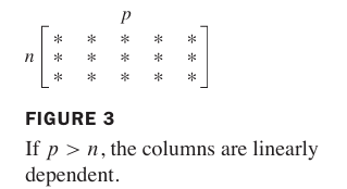
Example 5. The vectors \(\begin{bmatrix} 2 \\ 1 \end{bmatrix}, \begin{bmatrix} 4 \\ -1 \end{bmatrix}, \begin{bmatrix} -2 \\ 2 \end{bmatrix}\) are dependent because there are 3 vectors in \(\mathbb{R}^2\) (2 entries).

Theorem 9.: If a set \(S = \{\mathbf{v}_1, \dots, \mathbf{v}_p\}\) in \(\mathbb{R}^n\) contains the zero vector, then the set is linearly dependent.

Justification. \(1\cdot\mathbf{0} + 0\cdot\mathbf{v}_2 + \cdots + 0\cdot\mathbf{v}_p = \mathbf{0}\) gives a nontrivial relation.

Practice Problems (in‑class)

Describe the solution set of \(A\mathbf{x} = \mathbf{0}\) in parametric vector form, where \(A\) is row equivalent to

\[\begin{bmatrix} 1 & -2 & 0 & 3 \\ 0 & 1 & -4 & 0 \\ 0 & 0 & 0 & 0 \end{bmatrix}.\]
Let \(A\mathbf{x} = \mathbf{b}\) have the augmented matrix that reduces to

\[\left[\begin{array}{ccc|c} 1 & 0 & 2 & 3 \\ 0 & 1 & -1 & 1 \\ 0 & 0 & 0 & 0 \end{array}\right].\] Write the solution set in parametric vector form, and identify the particular solution and the solutions to \(A\mathbf{x} = \mathbf{0}\).
Are the vectors \(\begin{bmatrix} 1 \\ 0 \\ 2 \end{bmatrix}, \begin{bmatrix} -1 \\ 3 \\ 1 \end{bmatrix}, \begin{bmatrix} 5 \\ -6 \\ 0 \end{bmatrix}\) linearly independent? If not, find a dependence relation.
Give an example (by inspection) of three vectors in \(\mathbb{R}^3\) that are linearly dependent. Explain.
True or false: If \(\mathbf{v}_1, \mathbf{v}_2, \mathbf{v}_3\) are in \(\mathbb{R}^3\) and \(\mathbf{v}_3\) is not a linear combination of \(\mathbf{v}_1\) and \(\mathbf{v}_2\), then \(\{\mathbf{v}_1, \mathbf{v}_2, \mathbf{v}_3\}\) is linearly independent. Justify your answer.

(Solutions are at the end.)

R Supplement

Let’s use R to explore homogeneous solutions and linear independence.

# Example 1 (homogeneous) – row reduction to find solution
library(pracma)  # for reduced echelon form
A <- matrix(c(1, 1, -3,
              3, 4, -7,
             -5, -8, 9), nrow=3, byrow=FALSE)
b <- c(0, 0, 0)
aug <- cbind(A, b)
rref(aug)

            b
[1,] 1 0  4 0
[2,] 0 1 -3 0
[3,] 0 0  0 0

The reduced echelon form shows the free variable and the parametric vector.

# Example from practice problem 1 – give parametric solution
A2 <- matrix(c(1,0,0, -2,1,0, 0,-4,0, 3,0,0), nrow=3)
rref(cbind(A2, c(0,0,0)))

     [,1] [,2] [,3] [,4] [,5]
[1,]    1    0   -8    3    0
[2,]    0    1   -4    0    0
[3,]    0    0    0    0    0

# Solve: x1 = 8x2 - 3x4, x2 = 4x3, x3,x4 free

For linear independence:

# Example 1 (section 1.7): Check if columns are independent
A3 <- matrix(c(1,2,3, 4,5,6, 2,1,0), nrow=3)
rref(cbind(A3, c(0,0,0)))

     [,1] [,2] [,3] [,4]
[1,]    1    0   -2    0
[2,]    0    1    1    0
[3,]    0    0    0    0

# The presence of a free variable indicates dependence.
# Find a dependence relation
A3_reduced <- rref(cbind(A3, c(0,0,0)))
# last column gives relation: x1 = 2x3, x2 = -x3, choose x3=1 -> (2, -1, 1)

Solutions to Practice Problems

The reduced echelon form (from the given row equivalence) is essentially

\(\begin{bmatrix} 1 & -2 & 0 & 3 \\ 0 & 1 & -4 & 0 \\ 0 & 0 & 0 & 0 \end{bmatrix}\).

Augment with zero column. Reduce: \(R_1 \leftarrow R_1 + 2R_2\) gives \(\begin{bmatrix} 1 & 0 & -8 & 3 \\ 0 & 1 & -4 & 0 \\ 0 & 0 & 0 & 0 \end{bmatrix}\).

Variables: \(x_1,x_2\) basic, \(x_3,x_4\) free. Solution: \(x_1 = 8x_3 - 3x_4\), \(x_2 = 4x_3\). So

\[\mathbf{x} = x_3 \begin{bmatrix} 8 \\ 4 \\ 1 \\ 0 \end{bmatrix} + x_4 \begin{bmatrix} -3 \\ 0 \\ 0 \\ 1 \end{bmatrix}.\]
From the reduced matrix:

\[\begin{aligned} x_1 + 2x_3 &= 3 \\ x_2 - x_3 &= 1 \end{aligned}\] Basic: \(x_1,x_2\); free: \(x_3\). Solve: \(x_1 = 3 - 2x_3\), \(x_2 = 1 + x_3\).
Parametric form: \[\mathbf{x} = \begin{bmatrix} 3 \\ 1 \\ 0 \end{bmatrix} + x_3 \begin{bmatrix} -2 \\ 1 \\ 1 \end{bmatrix}.\] The particular solution is \(\mathbf{p} = (3,1,0)\), homogeneous solutions are multiples of \((-2,1,1)^T\).
Set up \(A\mathbf{x} = \mathbf{0}\):

\[\left[\begin{array}{ccc|c} 1 & -1 & 5 & 0 \\ 0 & 3 & -6 & 0 \\ 2 & 1 & 0 & 0 \end{array}\right] \sim \left[\begin{array}{ccc|c} 1 & -1 & 5 & 0 \\ 0 & 3 & -6 & 0 \\ 0 & 3 & -10 & 0 \end{array}\right] \sim \left[\begin{array}{ccc|c} 1 & -1 & 5 & 0 \\ 0 & 1 & -2 & 0 \\ 0 & 0 & -4 & 0 \end{array}\right].\] No free variables → only trivial solution → the vectors are linearly independent.
Choose vectors where one is a combination of others, e.g., \(\mathbf{v}_1 = \begin{bmatrix}1\\0\\0\end{bmatrix}\), \(\mathbf{v}_2 = \begin{bmatrix}0\\1\\0\end{bmatrix}\), \(\mathbf{v}_3 = \begin{bmatrix}2\\3\\0\end{bmatrix}\). \(\mathbf{v}_3 = 2\mathbf{v}_1 + 3\mathbf{v}_2\), so the set is dependent. (Any three vectors in \(\mathbb{R}^3\) with one being a linear combination of the others.)
False. It is possible that \(\mathbf{v}_3\) is not a combination of \(\mathbf{v}_1,\mathbf{v}_2\), but the set could still be dependent if \(\mathbf{v}_1\) and \(\mathbf{v}_2\) are dependent. However, the definition of linear dependence does not require that \(\mathbf{v}_3\) be a combination of the first two; it might be that \(\mathbf{v}_1\) is a combination of \(\mathbf{v}_2\) and \(\mathbf{v}_3\), for instance. So the statement is false. (Counterexample: \(\mathbf{v}_1 = \begin{bmatrix}0\\0\\0\end{bmatrix}\), \(\mathbf{v}_2 = \begin{bmatrix}1\\0\\0\end{bmatrix}\), \(\mathbf{v}_3 = \begin{bmatrix}0\\1\\0\end{bmatrix}\); \(\mathbf{v}_3\) is not a combination of \(\mathbf{v}_1,\mathbf{v}_2\), but the set is dependent because it contains the zero vector.)

Summary

Homogeneous systems always have the trivial solution; nontrivial solutions exist iff there are free variables.
The solution set of \(A\mathbf{x} = \mathbf{0}\) is a span of vectors (a line, plane, etc., through the origin).
The general solution of \(A\mathbf{x} = \mathbf{b}\) is a particular solution plus the homogeneous solution set (Theorem 6).
Linear independence means the only way to combine vectors to get \(\mathbf{0}\) is with all zero weights.
Linear independence of columns of \(A\) is equivalent to \(A\mathbf{x} = \mathbf{0}\) having only the trivial solution.
Sets with more vectors than entries, or containing the zero vector, are automatically dependent.
Next week we study linear transformations and their matrices.

Section 1.8 Introduction to Linear Transformations

Learning Objectives

After this lecture you will be able to:

Understand the vocabulary of transformations: domain, codomain, image, range.
Recognize that every matrix defines a transformation \(\mathbf{x} \mapsto A\mathbf{x}\) and that such transformations are linear.
Determine whether a given transformation is linear.
Find the standard matrix of a linear transformation from \(\mathbb{R}^n\) to \(\mathbb{R}^m\).
Apply geometric linear transformations (rotation, reflection, shear, projection) using their standard matrices.
Explain the concepts of “onto” and “one‑to‑one” for a linear transformation and relate them to pivot positions in the standard matrix.
Decide whether a linear transformation maps \(\mathbb{R}^n\) onto \(\mathbb{R}^m\) or is one‑to‑one by examining the standard matrix.

A transformation (or function or mapping) \(T\) from \(\mathbb{R}^n\) to \(\mathbb{R}^m\) is a rule that assigns to each vector \(\mathbf{x} \in \mathbb{R}^n\) a vector \(T(\mathbf{x}) \in \mathbb{R}^m\).
We write \(T: \mathbb{R}^n \to \mathbb{R}^m\).

The set \(\mathbb{R}^n\) is the domain of \(T\).
\(\mathbb{R}^m\) is the codomain.
For \(\mathbf{x} \in \mathbb{R}^n\), the vector \(T(\mathbf{x})\) is the image of \(\mathbf{x}\).
The set of all images \(T(\mathbf{x})\) is the range of \(T\).

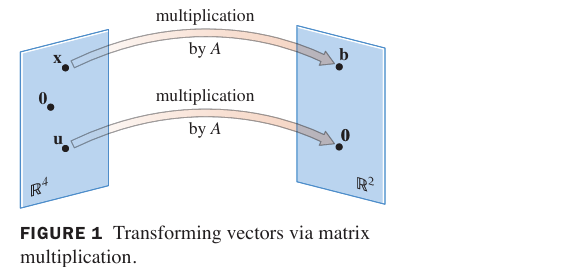
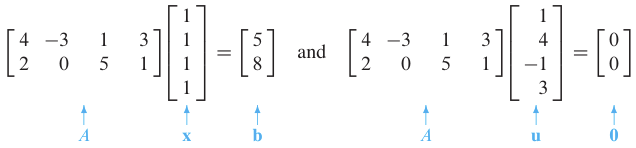
If \(A\) is an \(m \times n\) matrix, the rule \(T(\mathbf{x}) = A\mathbf{x}\) defines a transformation from \(\mathbb{R}^n\) to \(\mathbb{R}^m\). Such a transformation is called a matrix transformation, denoted by \(\mathbf{x} \mapsto A\mathbf{x}\). Here is the illustration,

For instance,

Example 1 (textbook). Let

\[A = \begin{bmatrix} 1 & -3 \\ 3 & 5 \\ -1 & 7 \end{bmatrix},\quad T(\mathbf{x}) = A\mathbf{x}.\]

This transformation \(T\) maps \(\mathbb{R}^2\) into \(\mathbb{R}^3\).
Given vectors \(\mathbf{u} = \begin{bmatrix}2\\-1\end{bmatrix}\), \(\mathbf{b} = \begin{bmatrix}3\\2\\-5\end{bmatrix}\), \(\mathbf{c} = \begin{bmatrix}3\\2\\5\end{bmatrix}\):

Find \(T(\mathbf{u}) :\)

\[T(\mathbf{u}) = A\mathbf{u} = \begin{bmatrix} 1(2) -3(-1) \\ 3(2) +5(-1) \\ -1(2) +7(-1) \end{bmatrix} = \begin{bmatrix}5\\1\\-9\end{bmatrix}.\]

Find an \(\mathbf{x}\) in \(\mathbb R^2\) whose image under \(T\) is \(\mathbf{b}\):

Solve \(A\mathbf{x} = \mathbf{b}\). By row-reducing the augmented matrix,

Row reduction yields a unique solution \(\mathbf{x} = \begin{bmatrix}1.5\\-0.5\end{bmatrix}\) (check: \(1.5\times 1 + (-0.5)\times(-3) = 3\), etc.).
Is there more than one \(\mathbf{x}\) whose image under \(T\) is \(\mathbf{b}\)? The solution is unique. (based on solving \(A\mathbf{x} = \mathbf{b}\) in b.)
Determine if \(\mathbf{c}\) is in the range of transformation \(T\):

Solve \(A\mathbf{x} = \mathbf{c}\). By row-reducing the augmented matrix,

The system is inconsistent (\(0=-35\) after row reduction), so \(\mathbf{c}\) is not in the range of transformation \(T\).

N.B. The vector \(\mathbf c\) is in the range of \(T\) if \(\mathbf c\) is the image of some \(\mathbf x\) in \(\mathbb R^2\), that is, if \(\mathbf c=T(\mathbf x)\) for some \(\mathbf x\). This is just another way of asking if the system \(A\mathbf x=\mathbf c\) is consistent.

N.B. This example illustrates that \(T(\mathbf{x}) = A\mathbf{x}\) transforms the question “is \(\mathbf{b}\) in the range?” into a system of linear equations.

Geometric examples: Projection and Shear Transformations

The following two matrix transformations can be viewed geometrically:

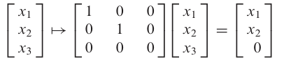
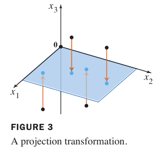
Projection: If \(A = \begin{bmatrix} 1 & 0 & 0 \\ 0 & 1 & 0 \\ 0 & 0 & 0 \end{bmatrix}\), the transformation \(\mathbf x \mapsto A\mathbf x\) maps (i.e., projects) points in \(\mathbb{R}^3\) onto the \(x_1x_2\)-plane, sending \(\begin{bmatrix}x_1\\x_2\\x_3\end{bmatrix} \mapsto \begin{bmatrix}x_1\\x_2\\0\end{bmatrix}\)
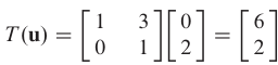
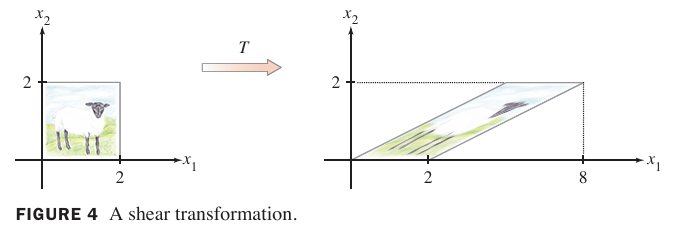
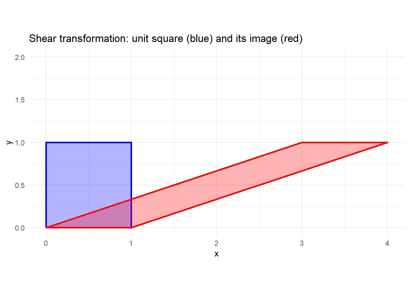
Shear: \(A = \begin{bmatrix} 1 & 3 \\ 0 & 1 \end{bmatrix}\) transforms the unit square into a parallelogram. (\(T: \mathbb R^2 \mapsto \mathbb R^2\)) The image of a point \((x_1,x_2)\) is \((x_1+3x_2,\; x_2)\). e.g.,

Parallelogram formed by shearing a square — Shear transformation of the unit square

Linear Transformations

Recall the theorem 5 in Section 1.4,

Theorem 5.

If \(A\) is \(m \times n\), \(\mathbf{u}, \mathbf{v} \in \mathbb{R}^n\), and \(c\) is a scalar, then

\(A(\mathbf{u} + \mathbf{v}) = A\mathbf{u} + A\mathbf{v}\)
\(A(c\mathbf{u}) = c(A\mathbf{u})\)

This theorem tells us the properties of transformation \(\mathbf x \mapsto A\mathbf x\). Now using function notation, we obtain

the definition of a linear transformation

A transformation (or mapping) \(T: \mathbb{R}^n \to \mathbb{R}^m\) is linear if for all \(\mathbf{u},\mathbf{v} \in \mathbb{R}^n\) and all scalars \(c\):

\(T(\mathbf{u} + \mathbf{v}) = T(\mathbf{u}) + T(\mathbf{v})\)
\(T(c\mathbf{u}) = c\,T(\mathbf{u})\)

Properties of linear transformations

If \(T\) is a linear transformation, then for all vectors \(\mathbf{u},\mathbf{v}\) in the domain of \(T\) and all scalars \(c,d\):

\(T(\mathbf{0}) = \mathbf{0}\) and
\(T(c\mathbf{u} + d\mathbf{v}) = cT(\mathbf{u}) + dT(\mathbf{v})\)
In general, \(T(c_1\mathbf{v}_1 + \cdots + c_p\mathbf{v}_p) = c_1 T(\mathbf{v}_1) + \cdots + c_p T(\mathbf{v}_p)\)

Proof.1.\(T(\mathbf{0}) = \mathbf{0}\) follows from \(T(0\mathbf{u}) = 0T(\mathbf{u})\).

Proof.2. Requires both conditions in the definition. (Set \(c=d=1\) for preservation of addition, and set \(d=0\) for preservation of scalar multiplication.)

Proof.3. Repeated application of property 2 produces the generalization.

N.B. If a transformation satisfies \(T(c\mathbf{u} + d\mathbf{v}) = cT(\mathbf{u}) + dT(\mathbf{v})\) for all \(\mathbf{u},\mathbf{v}\) and \(c,d\), it must be linear.

Linear transformations preserve the operations of vector addition and scalar multiplication. Equivalently, \(T(c_1\mathbf{v}_1 + c_2\mathbf{v}_2) = c_1 T(\mathbf{v}_1) + c_2 T(\mathbf{v}_2)\) for all \(\mathbf{v}_1,\mathbf{v}_2, c_1,c_2\).
This is called the superposition principle in engineering and physics.

Example 4 (textbook) – Contraction & Dilation. For a scalar \(r\), define \(T: \mathbb R^2 \mapsto \mathbb R^2\) by \(T(\mathbf{x}) = r\mathbf{x}\). Show that \(T\) is a linear transformation.

\(T\) is linear because

\[T(c\mathbf{u} + d\mathbf{v}) = r(c\mathbf{u} + d\mathbf{v}) = c(r\mathbf{u}) + d(r\mathbf{v}) = cT(\mathbf{u}) + dT(\mathbf{v}).\]

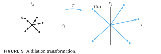
For transformation \(T(\mathbf{x}) = r\mathbf{x}\), \(T\) is called a contraction when \(0<r<1\) and a dilation when \(r>1\).

Rotation. The transformation that rotates every vector in \(\mathbb{R}^2\) counter‑clockwise by an angle \(\phi\) is linear. (We will find its matrix in Section 1.9.)

Example 5 (textbook) Rotation – Define a linear transformation \(T: \mathbb R^2 \mapsto \mathbb R^2\) by

Sol.

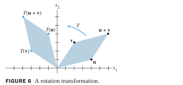
(Figure 6: \(T\) rotates \(\mathbf{u},\mathbf{v}\), and \(\mathbf{u} + \mathbf{v}\) counterclockwise about the origin through \(90^\circ\))

Check linearity experimentally using R. (optional)

# Verify linearity of rotation by 90 degrees
phi <- pi/2
A_rot <- matrix(c(cos(phi), sin(phi), -sin(phi), cos(phi)), nrow=2)
u <- c(2, 3)
v <- c(-1, 4)
c <- 2
d <- -0.5
T <- function(x) { A_rot %*% x }
left <- T(c*u + d*v)
right <- c*T(u) + d*T(v)
left

     [,1]
[1,] -4.0
[2,]  4.5

right

     [,1]
[1,] -4.0
[2,]  4.5

all.equal(left, right)

[1] TRUE

The output verifies that \(T(c\mathbf{u}+d\mathbf{v}) = cT(\mathbf{u}) + dT(\mathbf{v})\).

Remark: Every matrix transformation \(T(\mathbf{x}) = A\mathbf{x}\) is linear (Theorem 5 in Section 1.4). In \(\mathbb{R}^n\), every linear transformation is a matrix transformation (Section 1.9).

Section 1.9 The Matrix of a Linear Transformation

Learning Objectives

After this lecture you will be able to:

Find the standard matrix of a linear transformation from \(\mathbb{R}^n\) to \(\mathbb{R}^m\).
Apply geometric linear transformations (rotation, reflection, shear, projection) using their standard matrices.
Explain the concepts of “onto” and “one‑to‑one” for a linear transformation and relate them to pivot positions in the standard matrix.
Decide whether a linear transformation maps \(\mathbb{R}^n\) onto \(\mathbb{R}^m\) or is one‑to‑one by examining the standard matrix.

Every linear transformation \(T: \mathbb{R}^n \to \mathbb{R}^m\) can be represented as a matrix transformation.
The key is to look at the images of the standard basis vectors \(\mathbf{e}_1,\dots,\mathbf{e}_n\) (the columns of the \(n\times n\) identity matrix \(I_n\)).

Theorem 10

Theorem 10.: Let \(T: \mathbb{R}^n \to \mathbb{R}^m\) be a linear transformation. Then there exists a unique \(m\times n\) matrix \(A\) such that \[T(\mathbf{x}) = A\mathbf{x} \quad \text{for all } \mathbf{x}\in\mathbb{R}^n.\] In fact, the \(j\)‑th column of \(A\) is \(T(\mathbf{e}_j)\), where \(\mathbf{e}_j\) is the \(j\)‑th column of \(I_n\): \[A = \big[\, T(\mathbf{e}_1) \;\; T(\mathbf{e}_2) \;\; \cdots \;\; T(\mathbf{e}_n) \,\big].\]

The matrix \(A\) is called the standard matrix for the linear transformation \(T\).

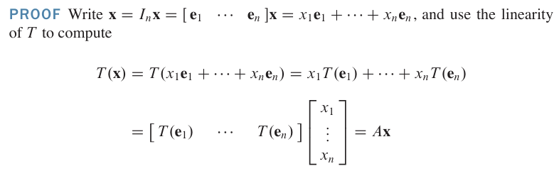
Example 1 (textbook). The columns of \(I_2\) are \(\mathbf{e}_1 = \begin{bmatrix}1\\0\end{bmatrix}\) and \(\mathbf{e}_2 = \begin{bmatrix}0\\1\end{bmatrix}\).
Suppose \(T: \mathbb{R}^2 \to \mathbb{R}^3\) is linear and

\[T(\mathbf{e}_1) = \begin{bmatrix}5\\-7\\2\end{bmatrix},\quad T(\mathbf{e}_2) = \begin{bmatrix}-3\\8\\0\end{bmatrix}.\] Find a formula for the image of an arbitrary \(\mathbf x\) in \(\mathbb R^2\).

Sol. For any \(\mathbf{x} = x_1\mathbf{e}_1 + x_2\mathbf{e}_2\), linearity gives

\[T(\mathbf{x}) = x_1 T(\mathbf{e}_1) + x_2 T(\mathbf{e}_2) = \begin{bmatrix} 5 & -3 \\ -7 & 8 \\ 2 & 0 \end{bmatrix} \begin{bmatrix} x_1 \\ x_2 \end{bmatrix}.\]

So the standard matrix is \(A = \begin{bmatrix} 5 & -3 \\ -7 & 8 \\ 2 & 0 \end{bmatrix}\).

N.B. Every linear transformation from \(\mathbb R^n\) to \(\mathbb R^m\) can be viewed as a matrix transformation, and vice versa. The term linear transformation focuses on a property of a mapping, while matrix transformation describes how such a mapping is implemented. (Example 2 & 3)

Example 2 (textbook) - Dilation. Find the standard matrix \(A\) for the \(T(\mathbf x)=3\mathbf x\).

Sol. By theorem 10,

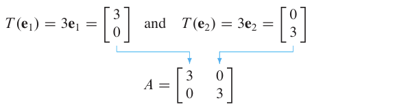
Example 3 (textbook) - counterclockwise rotation. Let \(T: \mathbb R^2 \mapsto \mathbb R^2\) be the transformation that rotates each point in \(\mathbb R^2\) about the origin through an angle \(\phi\), with counterclockwise rotation for a positive angle. Show geometrically that such a transformation is linear.

Sol.

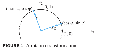
(Figure1 illustrates the rotation of basis vectors.)

For a rotation by angle \(\phi\),

\[\mathbf{e}_1 = \begin{bmatrix}1\\0\end{bmatrix} \mapsto \begin{bmatrix}\cos\phi\\ \sin\phi\end{bmatrix},\quad \mathbf{e}_2 = \begin{bmatrix}0\\1\end{bmatrix} \mapsto \begin{bmatrix}-\sin\phi\\ \cos\phi\end{bmatrix}.\]

Thus the standard matrix is \(\begin{bmatrix} \cos\phi & -\sin\phi \\ \sin\phi & \cos\phi \end{bmatrix}\).

Geometric Linear Transformations of \(\mathbb{R}^2\)

Using Theorem 10, we can write the standard matrix of common geometric transformations: Reflections, Projections, Shears, Contractions & Expansions.
(Refer to textbook Tables 1–4 for a complete list.)

Transformation	Standard matrix	Image of unit square
Reflection through \(x_1\)-axis	\(\begin{bmatrix} 1 & 0 \\ 0 & -1 \end{bmatrix}\)	mirrors vertically
Reflection through \(x_2\)-axis	\(\begin{bmatrix} -1 & 0 \\ 0 & 1 \end{bmatrix}\)	mirrors horizontally
Reflection through line \(x_1=x_2\)	\(\begin{bmatrix} 0 & 1 \\ 1 & 0 \end{bmatrix}\)	swaps axes
Reflection through line \(x_2=-x_1\)	\(\begin{bmatrix} 0 & -1 \\ -1 & 0 \end{bmatrix}\)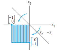
Reflection through the origin	\(\begin{bmatrix} -1 & 0 \\ 0 & -1 \end{bmatrix}\)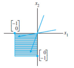
Projection onto \(x_1\)-axis	\(\begin{bmatrix} 1 & 0 \\ 0 & 0 \end{bmatrix}\)	flattens to a segment
Projection onto \(x_2\)-axis	\(\begin{bmatrix} 0 & 0 \\ 0 & 1 \end{bmatrix}\)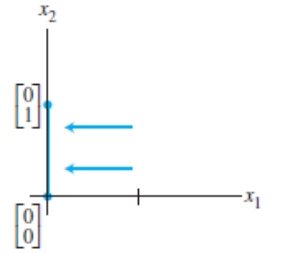
Horizontal shear	\(\begin{bmatrix} 1 & k \\ 0 & 1 \end{bmatrix}\)	pushes top edge right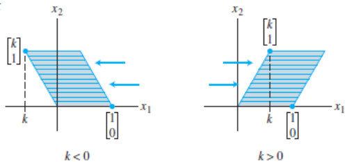
Vertical shear	\(\begin{bmatrix} 1 & 0 \\ k & 1 \end{bmatrix}\)	pushes right edge up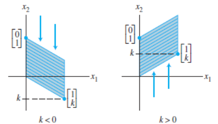
Horizontal Contraction and Expansion	\(\begin{bmatrix} k & 0 \\ 0 & 1 \end{bmatrix}\)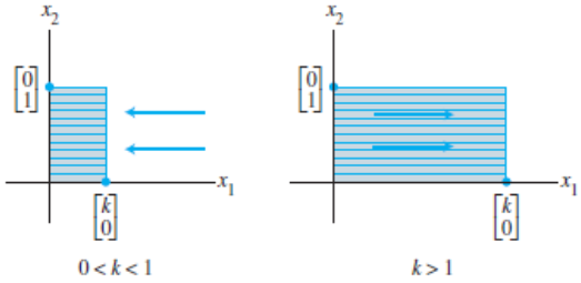
Vertical Contraction and Expansion	\(\begin{bmatrix} 1 & 0 \\ 0 & k \end{bmatrix}\)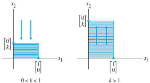
Rotation counter‑clockwise by \(\phi\)	\(\begin{bmatrix} \cos\phi & -\sin\phi \\ \sin\phi & \cos\phi \end{bmatrix}\)	rotates square
Dilation / contraction	\(\begin{bmatrix} r & 0 \\ 0 & r \end{bmatrix}\)	scales by \(r\)

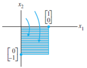
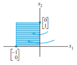
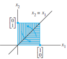
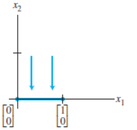
Onto and One‑to‑One Transformations

Definition

A transformation \(T: \mathbb{R}^n \to \mathbb{R}^m\) is onto \(\mathbb{R}^m\) if every \(\mathbf{b}\in\mathbb{R}^m\) is the image of at least one \(\mathbf{x}\in\mathbb{R}^n\). That is, the range of \(T\) is the whole codomain.

Equivalently, there exists at least one solution of \(T(\mathbf{x}) = \mathbf{b}\) for each \(\mathbf{b}\in\mathbb{R}^m\).

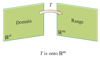
Interpretation: The mapping \(T\) is not onto when there is some \(\mathbf b\) in \(\mathbb{R}^m\) for which the equation \(T(\mathbf x)=\mathbf b\) has no solution.

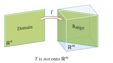
Definition

It is one‑to‑one if each \(\mathbf{b}\in\mathbb{R}^m\) is the image of at most one \(\mathbf{x}\in\mathbb{R}^n\).

Equivalently, for each \(\mathbf{b}\in\mathbb{R}^m\), the equation \(T(\mathbf x)=\mathbf b\) has has either a unique solution or none at all.

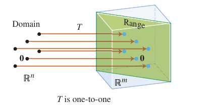
Interpretation: The mapping \(T\) is not one-to-one when some \(\mathbf{b}\in\mathbb{R}^m\) is the image of more than one vector in \(\mathbb{R}^n\).

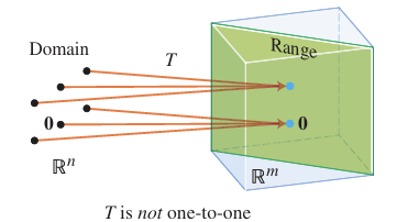
Theorem 11 & 12

Theorem 11: A linear transformation \(T: \mathbb{R}^n \to \mathbb{R}^m\) is one-to-one if and only if the equation \(T(\mathbf{x}) = \mathbf{0}\) has only the trivial solution.

N.B. For a linear transformation \(T(\mathbf{x}) = A\mathbf{x}\), these properties are read directly from the pivot structure of \(A\).

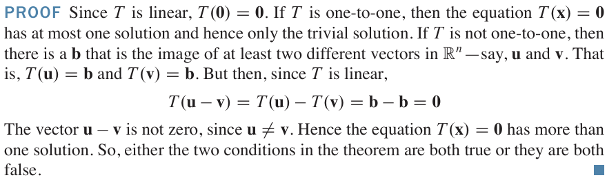
Theorem 12.

Let \(A\) be the standard matrix of \(T\).

\(T\) maps \(\mathbb{R}^n\) onto \(\mathbb{R}^m\) iff the columns of \(A\) span \(\mathbb{R}^m\) (i.e., \(A\) has a pivot in every row).
\(T\) is one‑to‑one iff the columns of \(A\) are linearly independent (i.e., \(A\mathbf{x}=\mathbf{0}\) has only the trivial solution – \(A\) has a pivot in every column).

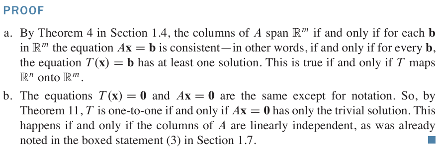
Example 4 (textbook). Let \(T\) be the linear transformation with standard matrix

\[A = \begin{bmatrix} 1 & -4 & 8 & 1 \\ 0 & 2 & -1 & 3 \\ 0 & 0 & 0 & 5 \end{bmatrix}.\] Does \(T\) map \(\mathbb R^4\)onto \(\mathbb R^3\)? Is \(T\) a one-to-one mapping?

Sol.

\(A\) has pivots in every row (3 pivots), so \(T\) is onto \(\mathbb{R}^3\).
\(A\) does not have a pivot in every column (4 columns, only 3 pivots), so \(T\) is not one‑to‑one (there is a free variable → equation \(T(\mathbf{x})=\mathbf{b}\) will have multiple solutions for each \(\mathbf{b}\) in the range).

Example 5 (textbook). Let \(T(x_1,x_2) = (3x_1 + x_2, 5x_1 + 7x_2, x_1 + 3x_2)\). Show \(T\) is a one-to-one mapping? Does \(T\) map \(\mathbb R^2\)onto \(\mathbb R^3\)?

Sol. Since

The standard matrix is

\[A = \begin{bmatrix} 3 & 1 \\ 5 & 7 \\ 1 & 3 \end{bmatrix}.\]

The columns of \(A\) are not multiples of each other; they are linearly independent. Hence \(T\) is one‑to‑one.
\(A\) is \(3\times 2\), so it cannot have a pivot in every row → \(T\) is not onto \(\mathbb{R}^3\). (The columns of \(A\) span \(\mathbb{R}^3\) if and only if it has 3 pivot positions.)

Practice Problems (in‑class)

Is the transformation \(T(x_1, x_2) = (3x_1 - x_2, \; |x_2|)\) linear? Why or why not?
Find the standard matrix of the linear transformation \(T: \mathbb{R}^2 \to \mathbb{R}^3\) defined by

\[T\left(\begin{bmatrix} x_1 \\ x_2 \end{bmatrix}\right) = \begin{bmatrix} 2x_1 - x_2 \\ x_1 + 4x_2 \\ -3x_1 \end{bmatrix}.\]
Let \(T\) be a linear transformation from \(\mathbb{R}^2\) to \(\mathbb{R}^2\) that first reflects points through the \(x_1\)‑axis and then rotates them by \(\pi/2\) counter‑clockwise. Find the standard matrix of this composite transformation. (Hint: multiplication of the corresponding matrices in the correct order.)
Determine whether the linear transformation \(T(\mathbf{x}) = A\mathbf{x}\) with \(A = \begin{bmatrix} 1 & -2 & 3 \\ 2 & -4 & 6 \end{bmatrix}\) is (a) onto \(\mathbb{R}^2\), (b) one‑to‑one.
Suppose \(T: \mathbb{R}^3 \to \mathbb{R}^4\) is linear and its standard matrix has 3 pivot columns and 4 rows. Is \(T\) onto \(\mathbb{R}^4\)? Is it one‑to‑one?

(Solutions appear at the end.)

R Supplement

We can build standard matrices and explore transformations.

# Standard matrix from prescribed images of e1, e2
T_e1 <- c(2, -1, 4)
T_e2 <- c(3, 0, -2)
A <- cbind(T_e1, T_e2)
A

     T_e1 T_e2
[1,]    2    3
[2,]   -1    0
[3,]    4   -2

# Applying to a vector
x <- c(5, -3)
A %*% x   # same as T(x)

     [,1]
[1,]    1
[2,]   -5
[3,]   26

Visualize a rotation:

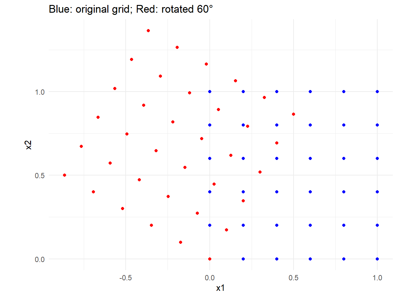
Check onto / one-to-one by pivots:

library(pracma)   # for rref
A_onto <- matrix(c(1,0,0, 0,1,0, -2,4,0, 1,0,3), nrow=3)
rref(A_onto)      # number of pivots = 3 (rows), so onto; but 4 columns => not one-to-one

     [,1] [,2] [,3] [,4]
[1,]    1    0   -2    0
[2,]    0    1    4    0
[3,]    0    0    0    1

A_12 <- matrix(c(1,2, -2,-4, 3,6), nrow=2)
rref(A_12)        # 1 pivot column, not all rows => not onto; columns dependent => not one-to-one

     [,1] [,2] [,3]
[1,]    1   -2    3
[2,]    0    0    0

Solutions to Practice Problems

Not linear. The presence of absolute value violates the scalar multiplication property: e.g., for \(c=-1\), \(T(-1\cdot(0,1)) = T(0,-1) = (1, 1)\), but \(-1\cdot T(0,1) = (1, -1)\). They are not equal.
Standard matrix is obtained by computing \(T(\mathbf{e}_1)\) and \(T(\mathbf{e}_2)\):

\[T(\mathbf{e}_1) = \begin{bmatrix}2\\1\\-3\end{bmatrix},\quad T(\mathbf{e}_2) = \begin{bmatrix}-1\\4\\0\end{bmatrix} \;\Rightarrow\; A = \begin{bmatrix} 2 & -1 \\ 1 & 4 \\ -3 & 0 \end{bmatrix}.\]
Reflection through \(x_1\)-axis: \(R = \begin{bmatrix} 1 & 0 \\ 0 & -1 \end{bmatrix}\). Rotation by \(\pi/2\): \(Q = \begin{bmatrix} 0 & -1 \\ 1 & 0 \end{bmatrix}\).
Composite: \(Q\,R = \begin{bmatrix} 0 & -1 \\ 1 & 0 \end{bmatrix} \begin{bmatrix} 1 & 0 \\ 0 & -1 \end{bmatrix} = \begin{bmatrix} 0 & 1 \\ 1 & 0 \end{bmatrix}\).
(This is reflection through the line \(x_1 = x_2\).)
Row reduce \(A\): \(\begin{bmatrix} 1 & -2 & 3 \\ 2 & -4 & 6 \end{bmatrix} \sim \begin{bmatrix} 1 & -2 & 3 \\ 0 & 0 & 0 \end{bmatrix}\).
- Not onto \(\mathbb{R}^2\) because row 2 has no pivot.
- Not one‑to‑one because there are free variables (columns 2 and 3 are not pivot columns).
\(T: \mathbb{R}^3 \to \mathbb{R}^4\), standard matrix is \(4\times 3\) with 3 pivots.
- The matrix has a pivot in every row? No, it has only 3 columns, so at most 3 pivots; but 4 rows, so there is a row without a pivot. Thus \(T\) is not onto \(\mathbb{R}^4\).
- The matrix has 3 pivot columns out of 3, so \(A\mathbf{x}=\mathbf{0}\) has only the trivial solution; thus \(T\) is one‑to‑one.

Summary

A transformation \(T: \mathbb{R}^n \to \mathbb{R}^m\) maps vectors from a domain to a codomain.
\(T\) is linear if it respects addition and scalar multiplication.
Every linear transformation from \(\mathbb{R}^n\) to \(\mathbb{R}^m\) can be written as \(T(\mathbf{x}) = A\mathbf{x}\), where the columns of \(A\) are the images of the standard basis vectors.
Geometric transformations (rotations, reflections, shears) are expressed by simple \(2\times 2\) matrices.
A linear transformation is onto if its standard matrix has a pivot in every row; it is one‑to‑one if the matrix has a pivot in every column.
These ideas connect the geometric concept of a transformation with the algebraic tool of matrix multiplication.

These notes follow Chapter 1 of Lay, Lay & McDonald, “Linear Algebra and its Applications”, 5th edition.