Perform matrix addition, scalar multiplication, and matrix multiplication.
Understand the non‑commutative nature of matrix multiplication and the conditions for product definition.
Compute powers and the transpose of a matrix.
We now extend the familiar arithmetic of vectors to matrices.
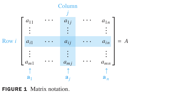
A matrix \(A\) is \(m\times n\); its \((i,j)\)‑entry is \(a_{ij}\). We often write \(A = [\mathbf{a}_1\; \mathbf{a}_2\; \dots\; \mathbf{a}_n]\) where the columns \(\mathbf{a}_j\) are vectors in \(\mathbb{R}^m\).
Matrix Basics: Diagonal, Triangular, and Zero Matrices
Main Diagonal and Diagonal Entries
For an \(m \times n\) matrix \[A = [a_{ij}],\] the diagonal entries are \[a_{11}, a_{22}, a_{33}, \dots\] and they form the main diagonal of \(A\).
Diagonal Matrix
A diagonal matrix is a square\(n \times n\) matrix in which all entries off the main diagonal are zero.
Example: the \(n \times n\)identity matrix\[I_n =
\begin{bmatrix}
1 & 0 & \cdots & 0 \\
0 & 1 & \cdots & 0 \\
\vdots & \vdots & \ddots & \vdots \\
0 & 0 & \cdots & 1
\end{bmatrix}\] which has diagonal entries equal to \(1\).
Zero Matrix
An \(m \times n\) matrix whose entries are all zero is called a zero matrix, denoted by \(\mathbf{0}\). Its size is usually clear from context.
Upper and Lower Triangular Matrices
An upper triangular matrix is a square matrix where all nonzero entries lie on or above the main diagonal: \[\begin{bmatrix}
a_{11} & a_{12} & \cdots & a_{1n} \\
0 & a_{22} & \cdots & a_{2n} \\
\vdots & \vdots & \ddots & \vdots \\
0 & 0 & \cdots & a_{nn}
\end{bmatrix} .\]
A lower triangular matrix is a square matrix where all nonzero entries lie on or below the main diagonal: \[\begin{bmatrix}
a_{11} & 0 & \cdots & 0 \\
a_{21} & a_{22} & \cdots & 0 \\
\vdots & \vdots & \ddots & \vdots \\
a_{n1} & a_{n2} & \cdots & a_{nn}
\end{bmatrix}.\]
Sums and Scalar Multiples
Two matrices are equal if they have the same size (i.e., the same number of rows and the same number of columns) and their corresponding entries are equal.
If \(A\) and \(B\) are both \(m\times n\), their sum\(A+B\) is the \(m\times n\) matrix whose entries are the sums of corresponding entries: \((A+B)_{ij}=a_{ij}+b_{ij}\).
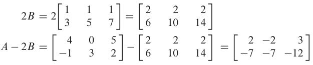
For a scalar \(r\), the scalar multiple\(rA\) is the matrix with entries \((rA)_{ij}=r\,a_{ij}\).
Example 1 & 2 (textbook).\[A=\begin{bmatrix} 4 & 0 & 5 \\ -1 & 3 & 2 \end{bmatrix},\quad
B=\begin{bmatrix} 1 & 1 & 1 \\ 3 & 5 & 7 \end{bmatrix},\quad
C=\begin{bmatrix} 2 & -3 \\ 0 & 1 \end{bmatrix}.\] Then \(A+B = \begin{bmatrix} 5 & 1 & 6 \\ 2 & 8 & 9 \end{bmatrix}\), but \(A+C\) is not defined because sizes differ.
Theorem 1 - Algebraic Properties
Theorem 1 (algebraic properties).
For matrices of the same size and scalars \(r,s\):
\(A+B = B+A\)
\((A+B)+C = A+(B+C)\)
\(A+0 = A\)
\(r(A+B) = rA+rB\)
\((r+s)A = rA+sA\)
\(r(sA) = (rs)A\)
Matrix Multiplication: Theory, Motivation, and Computation
N.B. The product \(AB\) is defined only when the number of columns of \(A\) equals the number of rows of \(B\).
Definition
If \(A\) is \(m\times n\) and \(B\) is \(n\times p\), with columns \(\mathbf{b}_1,\dots,\mathbf{b}_p\), then \[AB = A[\mathbf{b}_1\;\mathbf{b}_2\;\dots\;\mathbf{b}_p] = [A\mathbf{b}_1\; A\mathbf{b}_2\; \dots\; A\mathbf{b}_p].\] That is, the \(j\)‑th column of \(AB\) is the linear combination of the columns of \(A\) using the \(j\)‑th column of \(B\) as weights.
Motivation: The Composition of Linear Transformations
Why is matrix multiplication defined in such a seemingly complicated way? The answer lies in linear transformations.
Let \(A\) be an \(m \times n\) matrix. It defines a linear transformation that maps vectors in \(\mathbb{R}^n\) to vectors in \(\mathbb{R}^m\) via \(\mathbf{x} \mapsto A\mathbf{x}\).
Let \(B\) be an \(n \times p\) matrix. It maps vectors in \(\mathbb{R}^p\) to vectors in \(\mathbb{R}^n\) via \(\mathbf{x} \mapsto B\mathbf{x}\).
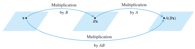
If we apply these transformations in sequence—first \(B\), then \(A\)—the resulting vector is: \[ A(B\mathbf{x}) \] This is a composition of two linear mappings.
Our goal is to find a single matrix that represents this overall composition. Let’s call this matrix \(AB\). We want it to satisfy: \[ (AB)\mathbf{x} = A(B\mathbf{x}) \tag{1} \] for every vector \(\mathbf{x}\) in \(\mathbb{R}^p\). This is the fundamental motivation behind the definition of matrix multiplication.
Deriving the Definition (The “Why”)
To see what \(AB\) must be, let’s break down the process.
Let \(B\) have columns \(\mathbf{b}_1, \mathbf{b}_2, \dots, \mathbf{b}_p\). So we write: \[ B = \begin{bmatrix} \mathbf{b}_1 & \mathbf{b}_2 & \cdots & \mathbf{b}_p \end{bmatrix} \] Let \(\mathbf{x}\) be any vector in \(\mathbb{R}^p\), with entries \(x_1, x_2, \dots, x_p\). By the definition of matrix-vector multiplication, the product \(B\mathbf{x}\) is a linear combination of the columns of \(B\): \[ B\mathbf{x} = x_1\mathbf{b}_1 + x_2\mathbf{b}_2 + \cdots + x_p\mathbf{b}_p \]
Now, multiply both sides on the left by \(A\): \[ A(B\mathbf{x}) = A\left(x_1\mathbf{b}_1 + x_2\mathbf{b}_2 + \cdots + x_p\mathbf{b}_p\right) \]
Because multiplication by a matrix is a linear operation, we can distribute \(A\) across the sum and pull out the scalar weights \(x_i\) (by theorem 5 in section 1.4): \[ A(B\mathbf{x}) = x_1 A\mathbf{b}_1 + x_2 A\mathbf{b}_2 + \cdots + x_p A\mathbf{b}_p \]
The expression on the right is a linear combination of the vectors \(A\mathbf{b}_1, A\mathbf{b}_2, \dots, A\mathbf{b}_p\), with weights \(x_1, \dots, x_p\). In matrix notation, a linear combination like this can be written as a matrix-vector product: \[ A(B\mathbf{x}) = \begin{bmatrix} A\mathbf{b}_1 & A\mathbf{b}_2 & \cdots & A\mathbf{b}_p \end{bmatrix} \mathbf{x} \]
Comparing this with equation (1), we see that the matrix we are looking for, \(AB\), is exactly: \[ AB = \begin{bmatrix} A\mathbf{b}_1 & A\mathbf{b}_2 & \cdots & A\mathbf{b}_p \end{bmatrix} \]
Thus, the product\(AB\) is formed by multiplying each column of \(B\) by \(A\) and using these resulting vectors as the columns of the new matrix.
Formal Definition
Definition: If \(A\) is an \(m \times n\) matrix and \(B\) is an \(n \times p\) matrix with columns \(\mathbf{b}_1, \dots, \mathbf{b}_p\), then the product \(AB\) is the \(m \times p\) matrix whose columns are \(A\mathbf{b}_1, \dots, A\mathbf{b}_p\): \[ AB = A\begin{bmatrix} \mathbf{b}_1 & \mathbf{b}_2 & \cdots & \mathbf{b}_p \end{bmatrix} = \begin{bmatrix} A\mathbf{b}_1 & A\mathbf{b}_2 & \cdots & A\mathbf{b}_p \end{bmatrix} \]
N.B. The number of columns of \(A\) must equal the number of rows of \(B\) (both are \(n\)), otherwise the products \(A\mathbf{b}_i\) are not defined.
Size check: If \(A\) is \(m \times n\) and \(B\) is \(n \times p\), then \(AB\) is \(m \times p\).
\(AB\) has the same number of rows as \(A\).
\(AB\) has the same number of columns as \(B\).
Row-Column Rule (practical hand calculation)
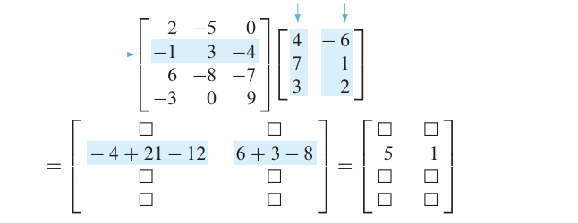
The \((i,j)\)‑entry of \(AB\) is the dot product of row \(i\) of \(A\) with column \(j\) of \(B\): \[(AB)_{ij} = a_{i1}b_{1j} + a_{i2}b_{2j} + \cdots + a_{in}b_{nj}.\]
N.B. A useful consequence of the row-column rule is the following general rule: \[\text{row}_i(AB) = \text{row}_i(A) \cdot B\] That is, the \(i\)-th row of the product is obtained by multiplying the \(i\)-th row of \(A\) by the entire matrix \(B\).
N.B. We say that \(A\) is right-multiplied by \(B\) when we compute \(AB\), or \(B\) is left-multiplied by \(A\).
Powers of a Matrix
If \(A\) is \(n\times n\), define \(A^k = \underbrace{A\cdots A}_{k\text{ times}}\) for positive integer \(k\).
We set \(A^0 = I_n\). Powers are useful for dynamic systems (later chapters).
The Transpose of a Matrix
The transpose of an \(m\times n\) matrix \(A\), written \(A^T\), is the \(n\times m\) matrix whose columns are the rows of \(A\): \((A^T)_{ij} = a_{ji}\).
Example 8 (textbook).\[A = \begin{bmatrix} a & b \\ c & d \end{bmatrix},\quad A^T = \begin{bmatrix} a & c \\ b & d \end{bmatrix}.\]
Theorem 3
Theorem 3.
Assume sizes are appropriate.
\((A^T)^T = A\)
\((A+B)^T = A^T + B^T\)
\((rA)^T = rA^T\)
\((AB)^T = B^T A^T\) (note the reversed order!)
Section 2.2 The Inverse of a Matrix
Learning Objectives
After this lecture you will be able to:
State the definition of an invertible matrix and its inverse.
Determine whether a \(2\times2\) matrix is invertible using the determinant.
Find the inverse of an invertible matrix using the row‑reduction algorithm \([A\;I]\sim[I\;A^{-1}]\).
Apply the inverse to solve a linear system \(A\mathbf{x}=\mathbf{b}\).
Relate elementary matrices to elementary row operations.
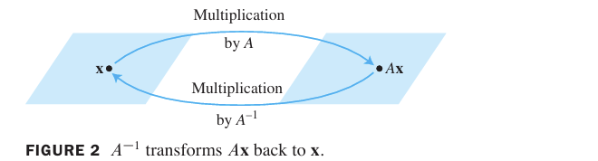
An \(n\times n\) matrix \(A\) is invertible if there exists an \(n\times n\) matrix \(C\) such that \[AC = I \quad\text{and}\quad CA = I.\] This \(C\) is unique; it is denoted \(A^{-1}\) and is called the inverse of \(A\). Therefore,
\[AA^{-1} = I \quad\text{and}\quad A^{-1}A = I.\]
A non‑invertible square matrix is singular; an invertible one is non‑singular.
Example 1 (textbook).
If \(A = \begin{bmatrix} 2 & 5 \\ -3 & -7 \end{bmatrix}\) and \(C = \begin{bmatrix} -7 & -5 \\ 3 & 2 \end{bmatrix}\), then
Let \(A = \begin{bmatrix} a & b \\ c & d \end{bmatrix}\). If \(ad-bc \neq 0\), then \(A\) is invertible and \[A^{-1} = \frac{1}{ad-bc}\begin{bmatrix} d & -b \\ -c & a \end{bmatrix}.\] If \(ad-bc = 0\), \(A\) is not invertible.
The number \(ad-bc\) is called the determinant of \(A\), written \(\det A\).
If \(A\) is an invertible \(n\times n\) matrix, then for any \(\mathbf{b}\in\mathbb{R}^n\) the equation \(A\mathbf{x}=\mathbf{b}\) has the unique solution \[\mathbf{x} = A^{-1}\mathbf{b}.\]
Proof.\(A(A^{-1}\mathbf{b}) = (AA^{-1})\mathbf{b} = I\mathbf{b} = \mathbf{b}\), so \(A^{-1}\mathbf b\) is a solution. If\(A\mathbf{u}=\mathbf{b}\), multiply both sides by \(A^{-1}\) on the left: \(\mathbf{u} = A^{-1}\mathbf{b}\), so the solution is unique.
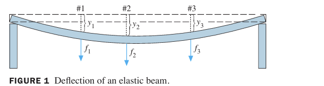
Example 3 (textbook). In an elastic beam deflection problem, a horizontal elastic beam is supported at each end and is subjected to forces at points 1, 2, and 3, as shown in Figure 1.
\(f \in \mathbb{R}^3\) list the downward forces at points 1, 2, and 3.
\(y \in \mathbb{R}^3\) list the resulting deflections (movements) at these points.
By Hooke’s law, the relationship is linear: \[y = Df\] where \(D\) is the flexibility matrix. Its inverse, \(D^{-1}\), is called the stiffness matrix.
Describe the physical significance of the columns of \(D\) and \(D^{-1}\).
Sol.
Physical Meaning of the Columns of\(D\) (Flexibility)
Recall the identity matrix \(I_3 = [\mathbf{e}_1 \ \mathbf{e}_2 \ \mathbf{e}_3]\). Since \(D = DI_3\), we have: \[D = [D\mathbf{e}_1 \quad D\mathbf{e}_2 \quad D\mathbf{e}_3]\]
The vector \(\mathbf{e}_1 = (1,0,0)\) represents a unit downward force applied only at point 1 (and zero force at points 2 and 3).
Therefore, column 1 of \(D\) (\(D\mathbf{e}_1\)) lists the deflections at all three points caused by that single unit force at point 1.
Similarly, column 2 of \(D\) gives the deflections due to a unit force at point 2, and column 3 gives deflections due to a unit force at point 3.
In short: Column \(j\) of \(D\) shows how the beam bends when a unit load (force) is placed exclusively at point \(j\).
Physical Meaning of the Columns of\(D^{-1}\) (Stiffness)
Now consider the inverse relationship: \[f = D^{-1}y\] Given a desired deflection pattern \(y\), this computes the required forces \(f\).
The vector \(\mathbf{e}_1 = (1,0,0)\) now represents a unit deflection at point 1, with zero deflection at points 2 and 3.
Thus, column 1 of \(D^{-1}\) lists the forces that must be applied at all three points to produce exactly that deflection pattern (unit deflection at point 1, none elsewhere).
Similarly, column 2 of \(D^{-1}\) gives the forces needed for a unit deflection at point 2, and column 3 for a unit deflection at point 3.
In short: The columns of \(D^{-1}\) give the forces needed to produce a unit deflection at a single point.
Notice that to achieve a unit deflection at one point while keeping the others fixed, some of the required forces may be negative (i.e., acting upward rather than downward).
Notes on Units:
If the flexibility matrix \(D\) is measured, for example, in inches of deflection per pound of force, then its inverse \(D^{-1}\) is measured in pounds of force per inch of deflection — which matches the intuitive meaning of stiffness.
Theorem 6 - Properties of the Inverse
Theorem 6.
If \(A\) and \(B\) are invertible \(n\times n\) matrices, then:
\((A^{-1})^{-1} = A\)
\((AB)^{-1} = B^{-1}A^{-1}\) (reverse order)
\((A^T)^{-1} = (A^{-1})^T\)
N.B. The product of invertible matrices is invertible, and the inverse is the product of the inverses in reverse order.
Proof.Proof Strategy (Verification by Definition): we rely on the defining criterion for an inverse:
A matrix \(X\) is the inverse of a matrix \(Y\) if and only if \[ XY = I \quad \text{and} \quad YX = I. \]Consequently, to prove that a proposed matrix is the inverse of a given matrix, it suffices to multiply the two matrices in both orders and verify that both products equal the identity matrix \(I\).
Proof of Part 1. The inverse of \(A^{-1}\) is \(A\).
Compute the products in both orders:
Right multiplication: \[ A^{-1} A = I. \]
Left multiplication: \[ A A^{-1} = I. \]
Since both products yield the identity matrix, \(A\) is indeed the inverse of \(A^{-1}\). Hence, \[ (A^{-1})^{-1} = A. \]
Proof of Part 2. The inverse of \(AB\) is \(B^{-1} A^{-1}\). (reverse order)
First, compute the product of \(AB\) with the candidate on the right: \[ (AB)(B^{-1} A^{-1}) = A (B B^{-1}) A^{-1} = A I A^{-1} = A A^{-1} = I. \]
Next, compute the product of the candidate with \(AB\) on the left: \[ (B^{-1} A^{-1})(AB) = B^{-1} (A^{-1} A) B = B^{-1} I B = B^{-1} B = I. \]
In both cases, the product equals \(I\). Therefore, by the defining criterion, \(B^{-1} A^{-1}\) is the inverse of \(AB\):
\[ (AB)^{-1} = B^{-1} A^{-1}. \]N.B. The order of multiplication must be reversed because matrix multiplication is generally non-commutative. If \(A\) and \(B\) do not commute, then \(A^{-1}B^{-1}\) would not, in general, invert \(AB\). The reverse order \(B^{-1}A^{-1}\) is the only correct form.
Proof of Part 3. The inverse of \(A^T\) is \((A^{-1})^T\).
We use the transpose property \((XY)^T = Y^T X^T\) (Theorem 3), and the fact that the identity matrix is symmetric, so \(I^T = I\).
First, multiply \((A^{-1})^T\) on the right by \(A^T\): \[ (A^{-1})^T A^T = (A A^{-1})^T = I^T = I. \]
Next, multiply \(A^T\) on the right by \((A^{-1})^T\): \[ A^T (A^{-1})^T = (A^{-1} A)^T = I^T = I. \]
Both products give the identity matrix. Hence, \((A^{-1})^T\) satisfies the definition of the inverse of \(A^T\):
\[ (A^T)^{-1} = (A^{-1})^T. \]
Elementary Matrices
An elementary matrix is obtained by performing a single elementary row operation on the identity matrix. There are three types:
Interchange:\(E = \begin{bmatrix} 1 & 0 & 0 \\ 0 & 0 & 1 \\ 0 & 1 & 0 \end{bmatrix}\)swap two rows (row 2 and row 3) of \(I\).
Scaling:\(E = \begin{bmatrix} 1 & 0 & 0 \\ 0 & 3 & 0 \\ 0 & 0 & 1 \end{bmatrix}\) multiply a row of \(I\) by a nonzero constant, e.g. multiply row 2 by 3.
N.B.Left-multiplying any matrix \(A\) by \(E\) (i.e., \(EA\)) performs that exact same row operation on \(A\). This is the core rule of How Elementary Matrices Work:
Rule: If an elementary row operation is performed on the identity matrix \(I_m\) to produce a matrix \(E\), then for any \(m \times n\) matrix \(A\), the product \(EA\) is precisely the result of applying that same row operation to \(A\).
Equivalently, the way\(E\) transforms \(A\) is determined entirely by how \(E\) was obtained from \(I\).
Why Does This Rule Hold?
To understand why, recall how matrix multiplication works at the row level. When we compute \(EA\):
Row\(i\) of \(EA\) is a linear combination of the rows of\(A\).
The coefficients for this linear combination are exactly the entries in row\(i\) of \(E\).
Now, since \(E\) was created from \(I_m\) by a specific row operation, the rows of \(E\) are simply the rows of \(I_m\) after that operation. But the rows of \(I_m\) are the standard basis vectors \(\mathbf{e}_1, \mathbf{e}_2, \dots, \mathbf{e}_m\). Therefore, the coefficients stored in the rows of \(E\) encode precisely the instructions for that operation.
When we multiply \(E\) by \(A\), those same coefficients combine the rows of \(A\) in exactly the same way.
Verifying this rule with Example 5 (textbook). Let
\[A = \begin{bmatrix} a & b & c \\ d & e & f \\ g & h & i \end{bmatrix}.\]
Compute \(E_1A\), \(E_2A\), and \(E_3A\), and describe how these products can be obtained by elementary row operations on \(A\).
Sol.
\[E_1A = \begin{bmatrix} a & b & c \\ d & e & f \\ g - 4a & h - 4b & i - 4c \end{bmatrix}, \quad
E_2A = \begin{bmatrix} d & e & f \\ a & b & c \\ g & h & i \end{bmatrix},\]
\[E_3A = \begin{bmatrix} a & b & c \\ d & e & f \\ 5g & 5h & 5i \end{bmatrix}.\]
Addition of \(-4\) times row 1 of \(A\) to row 3 produces \(E_1A\). (This is a row replacement operation.)
An interchange of rows 1 and 2 of \(A\) produces \(E_2A\).
Multiplication of row 3 of \(A\) by \(5\) produces \(E_3A\).
Left‑multiplication (that is, multiplication on the left) by \(E_1\) in Example 5 has the same effect on any \(3 \times n\) matrix. It adds \(-4\) times row 1 to row 3. In particular, since \(E_1 \cdot I = E_1\), we see that \(E_1\) itself is produced by this same row operation on the identity. Therefore,
If an elementary row operation is performed on an \(m \times n\) matrix \(A\), the resulting matrix can be written as \(EA\), where the \(m \times m\) matrix \(E\) is created by performing the same row operation on \(I_m\).
Example 6. Find the inverse of \(E = \begin{bmatrix} 1 & 0 & 0 \\ 0 & 1 & 0 \\ -4 & 0 & 1 \end{bmatrix}\).
Sol. To transform \(E\) into identity matrix, we add \(+4\)·row1 to row3. Therefore, the elementary matrix that does this is \(E^{-1} = \begin{bmatrix} 1 & 0 & 0 \\ 0 & 1 & 0 \\ 4 & 0 & 1 \end{bmatrix}\).
N.B. Every elementary matrix is invertible; its inverse is the elementary matrix that reverses the operation.
Algorithm for Finding \(A^{-1}\)
Theorem 7
Theorem 7.
An \(n\times n\) matrix \(A\) is invertible if and only if \(A\) is row equivalent to \(I_n\). In that case, any sequence of elementary row operations that reduces \(A\) to \(I_n\) also transforms \(I_n\) into \(A^{-1}\).
Remark on Logic: The phrase “if and only if” requires proving two implications:
If \(A\) is invertible, then \(A \sim I_n\) (the forward direction).
Conversely, if \(A \sim I_n\), then \(A\) is invertible (the reverse direction).
(The word “conversely” in the proof signals the start of the second implication.)
Proof.
the Forward Direction:\(A\) Invertible \(\Rightarrow\)\(A \sim I_n\). Assumption: \(A\) is an invertible \(n \times n\) matrix.
By Theorem 5 (the Invertible Matrix Theorem), the equation \[ A\mathbf{x} = \mathbf{b} \] has a solution for every vector \(\mathbf{b} \in \mathbb{R}^n\).
From Section 1.4 Theorem 4, we know that if a linear system \(A\mathbf{x} = \mathbf{b}\) is consistent for every choice of \(\mathbf{b}\), then \(A\) must have a pivot position in every row.
Since \(A\) is \(n \times n\), it has exactly \(n\) rows. Having a pivot in every row means there are \(n\) pivot positions in total. Because \(A\) is square, \(n\) pivot positions must occupy \(n\) distinct columns.
The only way to place \(n\) pivots in an \(n\)-column matrix without skipping any column is to have them on the main diagonal.
Therefore, the reduced row echelon form (RREF) of \(A\) has a leading \(1\) in every diagonal position and zeros elsewhere. That is exactly the identity matrix \(I_n\).
Thus, \(A\) is row equivalent to \(I_n\): \[ A \sim I_n. \]
the Converse Direction:\(A \sim I_n \Rightarrow A\) is Invertible (and later the Algorithm) Assumption: \(A\) is row equivalent to \(I_n\). That is, there is a finite sequence of elementary row operations that transforms \(A\) into \(I_n\).
Step 1: Translate row operations into matrix multiplications.
Let the row operations be applied in the order \(1, 2, \dots, p\). For each operation, there is a corresponding elementary matrix\(E_i\) such that left‑multiplying by \(E_i\) performs exactly that row operation. Therefore, the entire row reduction process can be written as: \[ E_p \cdots E_2 E_1 A = I_n. \tag{1} \]
Here: \(E_1\) corresponds to the first row operation, \(E_2\) corresponds to the second, and so on, the product \(E_p \cdots E_1\) represents the cumulative effect of all row operations.
Step 2: Show that the product of elementary matrices is invertible.
Each elementary matrix \(E_i\) is invertible (its inverse corresponds to the reverse row operation). The product of invertible matrices is also invertible. Hence, \[ M := E_p \cdots E_1 \] is an invertible matrix.
Step 3: Derive the inverse of \(A\).
From equation (1), we have \[ M A = I_n. \]
Since \(M\) is invertible, multiply both sides on the left by \(M^{-1}\): \[ M^{-1} (M A) = M^{-1} I_n. \] Using associativity, \((M^{-1}M) A = M^{-1}\), so \[ I_n A = M^{-1} \quad \Rightarrow \quad A = M^{-1}. \]
Because \(A\) is the inverse of the invertible matrix \(M\), \(A\) itself is invertible. Moreover, taking inverses on both sides gives: \[ A^{-1} = (M^{-1})^{-1} = M = E_p \cdots E_1. \tag{2} \]
Step 4: Connect this to the identity matrix.
Notice that \[ M I_n = M. \] But from (2), \(M = A^{-1}\). Therefore, \[ E_p \cdots E_1 I_n = A^{-1}. \]
This means that applying the same sequence of elementary matrices\(E_1, \dots, E_p\) to the identity matrix \(I_n\) yields exactly \(A^{-1}\).
N.B. Summary of the Converse Direction:
Since \(E_p \cdots E_1 A = I_n\), we have explicitly found a matrix \(M\) such that \(M A = I_n\). This proves invertibility.
The same \(M\) is equal to \(A^{-1}\).
Since \(M = E_p \cdots E_1\), applying those operations to \(I_n\) produces \(A^{-1}\).
This proof gives the practical algorithm for finding\(A^{-1}\):
Row reduce the augmented matrix\([A\; I]\). If \(A\) can be reduced to \(I\), then \([A\; I]\sim[I\; A^{-1}]\); otherwise \(A\) is not invertible.
Example 7 (textbook). Find the inverse of \(A = \begin{bmatrix} 0 & 1 & 2 \\ 1 & 0 & 3 \\ 4 & -3 & 8 \end{bmatrix}\)if it exists.
Computing \(A^{-1}\) explicitly and then multiplying \(\mathbf{b}\) is not the most efficient way to solve \(A\mathbf{x}=\mathbf{b}\). Row reduction directly on \([A\;\mathbf{b}]\) requires about \(1/3\) the operations of computing \(A^{-1}\) and \(A^{-1}\mathbf{b}\). In practice, the inverse is used mainly for theoretical analysis, not for solving systems.
Practice Problems (in‑class)
Let \(A = \begin{bmatrix} 1 & 3 \\ 2 & 5 \end{bmatrix}\), \(B = \begin{bmatrix} 1 & -1 \\ -1 & 2 \end{bmatrix}\). Compute \(AB\), \(BA\), and \((AB)^T\) to verify that \((AB)^T = B^T A^T\).
Determine whether \(A = \begin{bmatrix} 2 & 3 \\ 1 & 4 \end{bmatrix}\) is invertible. If so, find its inverse. (Hint: use Theorem 4.)
Use the inverse from Problem 2 to solve the system \[\begin{aligned}
2x_1 + 3x_2 &= 5 \\
x_1 + 4x_2 &= 6
\end{aligned}\]
Find the inverse of \(A = \begin{bmatrix} 1 & 0 & -2 \\ -3 & 1 & 4 \\ 2 & -3 & 4 \end{bmatrix}\) by row reducing \([A\; I]\). (You may check your answer with R.)
Which elementary matrix corresponds to interchanging rows 1 and 3 of a \(3\times 3\) matrix? What is its inverse?
(Solutions follow at the end.)
R Supplement
# Matrix operationsA <-matrix(c(2,3,1,-5), nrow=2, byrow=TRUE)B <-matrix(c(4,1,3,-2,6,3), nrow=2, byrow=TRUE) # note B is 2x3# Matrix multiplicationAB <- A %*% BAB
     [,1] [,2] [,3]
[1,]    2   20   15
[2,]   14  -29  -12
# Element-wise multiplication would be A * B (but not defined here)# Transpose and verify (AB)^T = B^T A^Tt(AB)
     [,1] [,2]
[1,]    2   14
[2,]   20  -29
[3,]   15  -12
t(B) %*%t(A)
     [,1] [,2]
[1,]    2   14
[2,]   20  -29
[3,]   15  -12
# Inverse of 2x2A2 <-matrix(c(2,3,1,4), nrow=2)det(A2)
[1] 5
A2_inv <-solve(A2)A2_inv
     [,1] [,2]
[1,]  0.8 -0.2
[2,] -0.6  0.4
# Solve linear system using inverseb <-c(5,6)x <- A2_inv %*% bx
     [,1]
[1,]  2.8
[2,] -0.6
# Inverse using augmented matrix [A|I] and row reductionlibrary(pracma) # for rrefA3 <-matrix(c(1,0,-2, -3,1,4, 2,-3,4), nrow=3, byrow=TRUE)aug <-cbind(A3, diag(3))rref_aug <-rref(aug)A3_inv <- rref_aug[,4:6]A3_inv
Interchange rows 1 and 3: \(E = \begin{bmatrix} 0 & 0 & 1 \\ 0 & 1 & 0 \\ 1 & 0 & 0 \end{bmatrix}\). Its inverse is itself because swapping twice returns to identity: \(E^{-1} = E\).
Summary
Matrix addition and scalar multiplication are entry‑wise operations.
Matrix multiplication is defined as \(A B\) when inner dimensions match; it corresponds to composition of linear transformations.
The transpose reverses rows and columns, and \((AB)^T = B^T A^T\).
An invertible matrix has an inverse \(A^{-1}\) satisfying \(AA^{-1} = I = A^{-1}A\).
For \(2\times2\) matrices, invertibility is determined by the determinant \(ad-bc\).
The inverse can be used to solve \(A\mathbf{x}=\mathbf{b}\) uniquely, but row reduction is more efficient.
Elementary matrices encode row operations and lead to the algorithm for computing \(A^{-1}\) via \([A\;I]\sim[I\;A^{-1}]\).
Section 2.3 Characterizations of Invertible Matrices
Learning Objectives
After this lecture you will be able to:
State the Invertible Matrix Theorem (IMT) for square matrices.
Understand the logical equivalence of all twelve statements in the theorem.
Use the IMT to determine whether a square matrix is invertible by checking just one of its equivalent conditions.
Explain how the IMT connects concepts from Chapter 1: linear systems, linear independence, spanning, and linear transformations.
Apply the IMT to decide whether a linear transformation \(\mathbf{x}\mapsto A\mathbf{x}\) is onto, one‑to‑one, or invertible.
Use the IMT to prove relationships between invertible matrices and related objects (e.g., transposes, products).
The Invertible Matrix Theorem (IMT) - Theorem 8
For a square \(n\times n\) matrix \(A\), many properties are all equivalent: either all are true or all are false. This powerful result gathers all the important characterizations of invertibility.
Theorem 8 (The Invertible Matrix Theorem).
Let \(A\) be an \(n\times n\) matrix. Then the following statements are equivalent.
\(A\) is an invertible matrix.
\(A\) is row equivalent to the \(n\times n\) identity matrix.
\(A\) has \(n\) pivot positions.
The equation \(A\mathbf{x} = \mathbf{0}\) has only the trivial solution.
The columns of \(A\) form a linearly independent set.
The linear transformation \(\mathbf{x}\mapsto A\mathbf{x}\) is one‑to‑one.
The equation \(A\mathbf{x} = \mathbf{b}\) has at least one solution for each \(\mathbf{b}\in\mathbb{R}^n\).
The columns of \(A\) span \(\mathbb{R}^n\).
The linear transformation \(\mathbf{x}\mapsto A\mathbf{x}\) maps \(\mathbb{R}^n\)onto\(\mathbb{R}^n\).
There is an \(n\times n\) matrix \(C\) such that \(CA = I\).
There is an \(n\times n\) matrix \(D\) such that \(AD = I\).
\(A^T\) is an invertible matrix.
Statements (m)–(r) give further equivalent conditions involving dimension and rank; they will be added in Section 2.9.
N.B.(g) Implies Unique Solutions:
Statement g. in the textbook says “The equation \(A\mathbf{x} = \mathbf{b}\) has at least one solution for each \(\mathbf{b}\) in \(\mathbb{R}^n\)”. In fact, it cannot have two or more solutions. We change the expression to make it clearer, that is, “g. The equation \(A\mathbf{x} = \mathbf{b}\) has exactly one solution for each \(\mathbf{b}\) in \(\mathbb{R}^n\)”. This statement certainly implies (b) and hence implies that \(A\) is invertible.
Why? Suppose \(A\mathbf{x} = \mathbf{b}\) had two solutions, \(\mathbf{x}_1\) and \(\mathbf{x}_2\). Then \(A(\mathbf{x}_1 - \mathbf{x}_2) = \mathbf{b} - \mathbf{b} = \mathbf{0}\). By (d), the only solution to the homogeneous equation is the zero vector, so \(\mathbf{x}_1 - \mathbf{x}_2 = \mathbf{0}\), meaning \(\mathbf{x}_1 = \mathbf{x}_2\). Thus, for an invertible matrix, every system \(A\mathbf{x} = \mathbf{b}\) has a unique solution.
Why is this theorem useful? To decide if a square matrix is invertible, you don’t need to compute its inverse; you can check any one of the equivalent conditions. For example, you can row reduce \(A\) to see if it has \(n\) pivots, or check if the columns are linearly independent, or see if \(A\mathbf{x}=\mathbf{0}\) has a nontrivial solution.
Proof outline
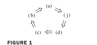
The proof establishes a circle of implications:
Then other statements are linked to this circle via earlier theorems.
\((a)\Rightarrow(j)\): Take \(C=A^{-1}\).
\((j)\Rightarrow(d)\): If \(CA=I\), then \(A\mathbf{x}=\mathbf{0}\) implies \(\mathbf{x}=I\mathbf{x}=CA\mathbf{x}=C\mathbf{0}=\mathbf{0}\).
\((d)\Rightarrow(c)\): If \(A\mathbf{x}=\mathbf{0}\) has only the trivial solution, then every column is a pivot column, so \(n\) pivots.
\((c)\Rightarrow(b)\): If \(A\) is square and has \(n\) pivot positions, then the pivots must lie on the main diagonal, where the reduced echelon form of A is \(I_n\):
\((b)\Rightarrow(a)\): If \(A\sim I\), by Theorem 7 in section 2.2, \(A\) is invertible.
The remaining connections rely on earlier theorems:
\((d)\Leftrightarrow(e)\Leftrightarrow(f)\) from Section 1.7 and Theorem 12(b) in section 1.9.
\((g)\Leftrightarrow(h)\Leftrightarrow(i)\) from Theorem 4 in Section 1.4 and Theorem 12(a) in Section 1.9.
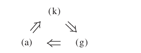
\((a)\Rightarrow(k)\), If \(A\) is invertible, then by definition, its inverse \(A^{-1}\) exists. we simply choose \(D=A^{-1}\), then \(AD = I\).
\((k)\Rightarrow(g)\), Construct a candidate solution: Let \(\mathbf{x} = D\mathbf{b}\). Now multiply both sides on the left by \(A\), \(A\mathbf{x} = A(D\mathbf{b})\). Because matrix multiplication is associative, we can regroup \(A(D\mathbf{b}) = (AD)\mathbf{b}\). But by assumption (k), \(AD = I\). Therefore \((A D)\mathbf{b} = I\mathbf{b} = \mathbf{b}\). So we have found an explicit vector \(\mathbf{x} = D\mathbf{b}\) that satisfies \(A\mathbf{x} = \mathbf{b}\). Since \(\mathbf{b}\) was arbitrary, the equation has a solution for every \(\mathbf{b} \in \mathbb{R}^n\). Thus, (k) implies (g).
\((g)\Rightarrow(a)\), Assume \(A\mathbf{x} = \mathbf{b}\) is consistent for every \(\mathbf{b}\). Let \(R\) be the reduced row echelon form (RREF) of \(A\). It is obvious that \(R\) has no zero rows. (Because if \(R\) had a row of all zeros, say the last row, then choosing \(\mathbf{b}\) with a non-zero entry in its last coordinate (e.g., \(\mathbf{b} = (0,0,\dots,0,1)^T\)) would make the system inconsistent, because the zero row corresponds to the equation \(0 = 1\). This contradicts our assumption.)
Since \(A\) is an \(n \times n\) matrix, it has exactly \(n\) rows. Having a pivot in every row means there are \(n\) pivot positions. Because there are only \(n\) columns, these \(n\) pivots must lie on the main diagonal. The only \(n \times n\) RREF matrix with a pivot in every row and every column is the identity matrix \(I_n\). So \(A \sim I_n\).
By the theorem we already proved (row equivalence to\(I_n\)implies invertibility), i.e., \((b)\Rightarrow(a)\), there exist elementary matrices \(E_1, \dots, E_p\) such that: \[E_p \cdots E_1 A = I_n.\] Let \(M = E_p \cdots E_1\). Then \(M A = I_n\). Since each elementary matrix is invertible, their product \(M\) is invertible. Multiplying on the left by \(M^{-1}\) gives: \[A = M^{-1}.\] Thus \(A\) is the inverse of an invertible matrix, hence \(A\) itself is invertible.
\((a)\Leftrightarrow(l)\) because of Theorem 6 (3.) in Section 2.2, and in this theorem the role of \(A\) and \(A^T\) are interchangeable.
Thus all twelve statements stand or fall together.
The “Square Inverse” Corollary
There is a very useful algebraic consequence of the IMT:
Fact
Let \(A\) and \(B\) be square matrices of the same size. If \(AB = I\), then both \(A\) and \(B\) are invertible, and they are inverses of each other (\(B = A^{-1}\) and \(A = B^{-1}\)).
Proof. If \(AB = I\), then \(B\) is a right inverse of \(A\). This is exactly statement (k) of the IMT. Since (k) implies (a), \(A\) is invertible. Now multiply both sides of \(AB = I\) on the left by \(A^{-1}\): \[ A^{-1}(AB) = A^{-1}I \quad \Rightarrow \quad (A^{-1}A)B = A^{-1} \quad \Rightarrow \quad I B = A^{-1} \quad \Rightarrow \quad B = A^{-1}. \] A similar argument shows \(A = B^{-1}\).
N.B. This fact is exceptionally useful because it means you only need to check multiplication in one order to confirm invertibility, provided the matrices are square.
Singular vs. Nonsingular Matrices
The Invertible Matrix Theorem divides the set of all \(n \times n\) matrices into two mutually exclusive classes:
Nonsingular (Invertible) Matrices: Matrices that satisfy all statements of the IMT.
Singular (Noninvertible) Matrices: Matrices that satisfy none of the invertibility properties.
Interpretations: If a matrix is singular,
it is not row equivalent to \(I_n\),
it has fewer than\(n\) pivot positions,
its columns are linearly dependent,
the transformation \(\mathbf{x} \mapsto A\mathbf{x}\) is not one-to-one and not onto.
the equation \(A\mathbf{x} = \mathbf{b}\) does not have a solution for every \(\mathbf{b}\).
In short, the negation of any single statement in the IMT automatically implies the negation of all the others.
Example 1 (textbook). Use the IMT to decide if \(A = \begin{bmatrix} 1 & 0 & -2 \\ 3 & 1 & -2 \\ -5 & -1 & 9 \end{bmatrix}\) is invertible.
The single most important limitation of the Invertible Matrix Theorem is that it only applies to square matrices (\(n \times n\)).
Do not apply the IMT to rectangular matrices!
For example, consider a \(4 \times 3\) matrix with linearly independent columns. Since it has 3 pivot positions (one in each column) and 4 rows, the columns are linearly independent. However, because it is not square, we cannot use the IMT to conclude anything about the existence of solutions to \(A\mathbf{x} = \mathbf{b}\).
N.B. Always check the dimensions before applying the IMT.
Invertible linear transformation
Just as we can invert a matrix, we can also invert a linear transformation. This extends the concept of invertibility to mappings.
Definition of Invertible Transformation
A linear transformation \(T: \mathbb{R}^n \to \mathbb{R}^n\) is said to be invertible if there exists a function \(S: \mathbb{R}^n \to \mathbb{R}^n\) such that:
\(S(T(\mathbf{x})) = \mathbf{x}\) for all \(\mathbf{x} \in \mathbb{R}^n\). (Applying\(T\) and then \(S\) returns the original vector.)
\(T(S(\mathbf{x})) = \mathbf{x}\) for all \(\mathbf{x} \in \mathbb{R}^n\). (Applying\(S\) and then \(T\) returns the original vector.)
If such an \(S\) exists, it is unique and must be a linear transformation (Theorem 9). It is called the inverse of \(T\), denoted by \(T^{-1}\).
Theorem 9: Invertible Transformations and Invertible Matrices
The connection between invertible matrices and invertible transformations is seamless.
Theorem 9
Let \(T: \mathbb{R}^n \to \mathbb{R}^n\) be a linear transformation, and let \(A\) be its standard matrix. Then:
\(T\) is invertible if and only if\(A\) is an invertible matrix.
In that case, the inverse transformation \(S(\mathbf{x}) = A^{-1}\mathbf{x}\) is the unique inverse of \(T\).
Proof.
We must prove both directions of the “if and only if.”
Part 1: If \(T\) is invertible, then \(A\) is invertible.
Assume \(T\) has an inverse \(S\). We want to show \(A\) satisfies the IMT. By definition of an inverse, \(T(S(\mathbf{x})) = \mathbf{x}\) for all \(\mathbf{x}\). This means that for any vector \(\mathbf{b} \in \mathbb{R}^n\), if we set \(\mathbf{x} = S(\mathbf{b})\), then \(T(\mathbf{x}) = T(S(\mathbf{b})) = \mathbf{b}\). This proves that \(T\) maps \(\mathbb{R}^n\)onto\(\mathbb{R}^n\) (every \(\mathbf{b}\) is hit by some input).
Since \(T\) is onto, \(A\) is invertible by statement (i) of the IMT.
Part 2: If \(A\) is invertible, then \(T\) is invertible.
Assume \(A\) is invertible, so \(A^{-1}\) exists. Define a new transformation \(S\) by \(S(\mathbf{x}) = A^{-1}\mathbf{x}\). We must verify \(S\) satisfies the properties of an inverse:
Check \(T(S(\mathbf{x}))\): \[ T(S(\mathbf{x})) = T(A^{-1}\mathbf{x}) = A(A^{-1}\mathbf{x}) = (AA^{-1})\mathbf{x} = I\mathbf{x} = \mathbf{x}. \] Because \(S\) satisfies both criteria, \(T\) is invertible, and \(S\) is its inverse \(T^{-1}\).
Example 2 (textbook). What can you say about a one-to-one linear transformation \(T: \mathbb{R}^n \to \mathbb{R}^n\)? (N.B. A One-to-One Transformation Must be Invertible. )
Sol. Let \(A\) be the standard matrix of \(T\).
Since \(T\) is one-to-one, the columns of \(A\) are linearly independent. (By Theorem 12 in Section 1.9, the columns of \(A\) are linearly independent if and only if the transformation \(T\) is one-to-one.)
Since \(A\) is square, all other statements of the IMT hold. Therefore, \(A\) is invertible. (This is statement (e) of the Invertible Matrix Theorem.)
By Theorem 9, if the standard matrix is invertible, the linear transformation \(T\) is invertible.
N.B. Conclusion: A one-to-one linear transformation from \(\mathbb{R}^n\) to \(\mathbb{R}^n\) is automatically onto\(\mathbb{R}^n\) and is invertible. This beautifully illustrates the power of the IMT: you only need to check “one-to-one” to guarantee “onto” and “invertible” for transformations on finite-dimensional spaces of equal dimension.
Numerical note
In practice, a matrix may be “nearly singular” (ill‑conditioned). When its condition number is large, the matrix is theoretically invertible but may behave like a singular matrix in finite‑precision arithmetic. Some computer programs compute the condition number to detect such situations.
Practice Problems (in‑class)
Determine if the matrix is invertible. Justify your answer using the IMT.
Suppose \(A\) is a \(5\times5\) matrix and the equation \(A\mathbf{x}=\mathbf{b}\) has a solution for every \(\mathbf{b}\in\mathbb{R}^5\). What can you say about the columns of \(A\)? What can you say about the equation \(A\mathbf{x}=\mathbf{0}\)? (Use IMT.)
If \(A\) is an \(n\times n\) matrix and the linear transformation \(\mathbf{x}\mapsto A\mathbf{x}\) is one‑to‑one, show that \(A\) is invertible.
True or False: If \(A\) is an invertible \(n\times n\) matrix, then the rows of \(A\) form a linearly independent set. Justify. (Hint: use statement (l) about \(A^T\).)
Let \(A\) and \(B\) be \(n\times n\) matrices such that \(AB\) is invertible. Prove that \(A\) and \(B\) are both invertible. (Hint: apply the IMT to \(AB\), then use statements (j) and (k) or argue via the determinant; the IMT provides several paths.)
(Solutions at the end.)
R Supplement
Check the IMT in action using R. We can row reduce to count pivots, test if a matrix is invertible via solve(), and verify equivalent statements.
library(pracma)# Example: a 3x3 matrixA <-matrix(c(1,2,3, 2,3,4, 3,4,5), nrow=3)# Row reduce to echelon form to count pivotsrrefA <-rref(A)rrefA
     [,1] [,2] [,3]
[1,]    1    0   -1
[2,]    0    1    2
[3,]    0    0    0
# Number of pivots (nonzero rows)sum(rowSums(abs(rrefA)) >1e-10) # less than 3 => not invertible
[1] 2
# Another matrix that is invertibleA2 <-matrix(c(1,0,-2, 3,1,-2, -5,-1,9), nrow=3)rrefA2 <-rref(A2)rrefA2
     [,1] [,2] [,3]
[1,]    1    0    0
[2,]    0    1    0
[3,]    0    0    1
# All rows nonzero => invertible# Solve A2 x = b for random bb <-c(2, -1, 3)x <-solve(A2, b)x
[1] 12.333333 2.666667 3.666667
# Check trivial solution of homogeneous equationx0 <-solve(A2, c(0,0,0))x0 # should be (0,0,0)
[1] 0 0 0
# Verify that inverse exists and product gives identityA2_inv <-solve(A2)A2_inv %*% A2 # identity
By IMT, statement (g) is equivalent to (a)–(l). So if \(A\mathbf{x}=\mathbf{b}\) has a solution for every \(\mathbf{b}\), then \(A\) is invertible. Consequently, the columns of \(A\) span \(\mathbb{R}^5\) and are linearly independent (IMT(h) and (e)). The equation \(A\mathbf{x}=\mathbf{0}\) has only the trivial solution (IMT(d)).
If \(\mathbf{x}\mapsto A\mathbf{x}\) is one‑to‑one, then by IMT statement (f) \(\Rightarrow\) (a), \(A\) is invertible. (Alternatively, one‑to‑one means \(A\mathbf{x}=\mathbf{0}\) has only the trivial solution, so (d) holds, which implies (a).)
True. By IMT, \(A\) invertible \(\Rightarrow\)\(A^T\) invertible (statement (l)). Then columns of \(A^T\) (which are the rows of \(A\)) are linearly independent (IMT(e) applied to \(A^T\)). So the rows of \(A\) form a linearly independent set.
Since \(AB\) is invertible, by IMT there exists a matrix \(W\) such that \((AB)W = I\). So \(A(BW) = I\). This shows \(A\) has a right inverse \(D = BW\), so by IMT statement (k) \(\Rightarrow\) (a), \(A\) is invertible. Similarly, from the other side \((W' )AB = I\) there is a left inverse for \(B\), so \(B\) is invertible. (A quicker argument: invertible product implies both factors are square and invertible via IMT.)
Alternative proof: Because \(AB\) is invertible, \(\det(AB)=\det A\det B\neq 0\), so both \(\det A\) and \(\det B\) are nonzero, hence \(A\) and \(B\) are invertible. (Determinants are not introduced until Chapter 3, but it’s a concise argument for later.)
Summary
The Invertible Matrix Theorem gives a dozen equivalent ways to say a square matrix is invertible.
You can determine invertibility by checking any one condition: pivot count, trivial solution to \(A\mathbf{x}=\mathbf{0}\), column independence, spanning, etc.
The theorem unifies earlier concepts (linear independence, span, one‑to‑one, onto) under the umbrella of invertibility.
It provides a powerful tool for proving relationships between matrices and linear transformations without heavy computation.
Next week we study subspaces, basis, dimension, and rank—extending the IMT even further.
Section 2.8 Subspaces of \(\mathbb R\)ⁿ
Learning Objectives
After this lecture you will be able to:
State the three properties that define a subspace of \(\mathbb{R}^n\).
Verify whether a given subset of \(\mathbb{R}^n\) is a subspace.
Define the column space and null space of a matrix.
Determine whether a vector belongs to \(\operatorname{Col} A\) or \(\operatorname{Nul} A\).
Use parametric vector form to produce an explicit description of \(\operatorname{Nul} A\).
Find a basis for \(\operatorname{Col} A\) (pivot columns of \(A\)) and for \(\operatorname{Nul} A\) (vectors from parametric solution).
Explain the relationship between pivot columns and a basis for the column space.
Subspaces
Definition
A subspace of \(\mathbb{R}^n\) is a set \(H \subseteq \mathbb{R}^n\) that satisfies three conditions:
The zero vector \(\mathbf{0}\) is in \(H\).
For every \(\mathbf{u},\mathbf{v} \in H\), the sum \(\mathbf{u}+\mathbf{v}\) is in \(H\). (\(H\) is closed under addition.)
For every \(\mathbf{u}\in H\) and every scalar \(c\), the vector \(c\mathbf{u}\) is in \(H\). (\(H\) is closed under scalar multiplication.)
In words: a subspace is a set of vectors in \(\mathbb{R}^n\) that is closed under linear combinations (addition and scalar multiplication).
Example 1 (textbook) – Span is a subspace. If \(\mathbf{v}_1\) and \(\mathbf{v}_2\) are in \(\mathbb{R}^n\) and \(H = \text{Span}\{\mathbf{v}_1, \mathbf{v}_2\}\), then \(H\) is a subspace of \(\mathbb{R}^n\).
First verify that the zero vector is in \(H\) because \(0\mathbf{v}_1 + 0\mathbf{v}_2\) is a linear combination of \(\mathbf{v}_1\) and \(\mathbf{v}_2\).
Example 3 (textbook) – The previous example generalizes naturally. For \(\mathbf{v}_1, \ldots, \mathbf{v}_p\) in \(\mathbb{R}^n\), the set of all linear combinations, \(H = \operatorname{Span}\{\mathbf{v}_1,\dots,\mathbf{v}_p\}\), is a subspace of \(\mathbb{R}^n\). We shall now refer to \(\text{Span} \{\mathbf{v}_1, \ldots, \mathbf{v}_p\}\) as the subspace spanned (or generated) by \(\mathbf{v}_1, \ldots, \mathbf{v}_p\).
Proof outline:
The zero vector is in \(H\) because \(\mathbf{0}=0\mathbf{v}_1+\cdots+0\mathbf{v}_p \in H\)
\(H\) is closed under addition: sums of linear combinations are again linear combinations.
\(H\) is closed under scalar multiplication: scalar multiples of linear combinations are again linear combinations.
N.B. In general, if \(\mathbf{v}_1,\dots,\mathbf{v}_p \in \mathbb{R}^n\), then \(H = \operatorname{Span}\{\mathbf{v}_1,\dots,\mathbf{v}_p\}\) is a subspace.
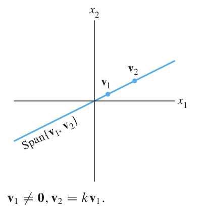
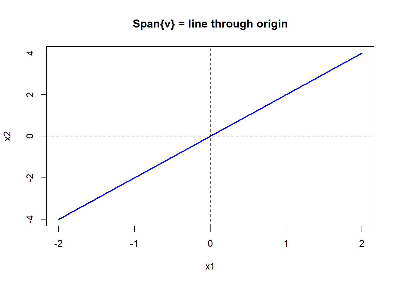
N.B. Thus every line through the origin and every plane through the origin is a subspace.
Code
x <-seq(-2,2,length=100)plot(x, 2*x, type='l', lwd=2, col='blue', xlab='x1', ylab='x2',main='Span{v} = line through origin')abline(h=0, v=0, lty=2)
A line through the origin is a subspace.
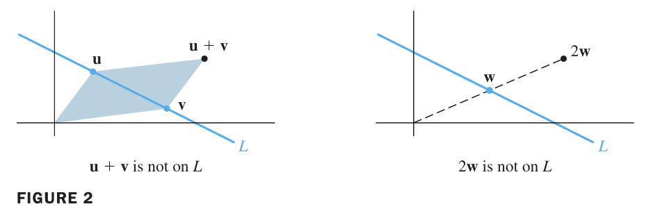
Example 2 (textbook) – A line NOT through the origin is NOT a subspace. It fails condition (a) because \(\mathbf{0}\) is not on the line, and also fails closure under addition.
N.B.The whole space\(\mathbb{R}^n\) is a subspace of itself. The zero subspace\(\{\mathbf{0}\}\) is a subspace (trivially).
Column Space and Null Space of a Matrix
Two fundamental subspaces associated with any \(m\times n\) matrix \(A\):
Column Space
The column space of \(A\), written \(\operatorname{Col} A\), is the set of all linear combinations of the columns of \(A\).
If \(A = [\mathbf{a}_1 \cdots \mathbf{a}_n]\), with columns in \(\mathbb{R}^m\), then \(\operatorname{Col} A = \operatorname{Span}\{\mathbf{a}_1,\dots,\mathbf{a}_n\}\).
N.B. Because it’s a span, \(\operatorname{Col} A\)is automatically a subspace of\(\mathbb{R}^m\) (since columns are in \(\mathbb{R}^m\)). \(\operatorname{Col} A\) equals \(\mathbb{R}^m\) only when the columns of \(A\) span \(\mathbb{R}^m\).
N.B.The equation\(A\mathbf{x} = \mathbf{b}\)has a solutioniff\(\mathbf{b} \in \operatorname{Col}A\), that is, the equivalence holds:
\(\mathbf{b} \in \operatorname{Col} A \quad \Longleftrightarrow \quad A\mathbf{x} = \mathbf{b} \text{ is consistent.}\)
Why? Let the columns of \(A\) be \(\mathbf{a}_1, \mathbf{a}_2, \dots, \mathbf{a}_n\). By definition:
\[\operatorname{Col} A = \operatorname{Span}\{\mathbf{a}_1, \mathbf{a}_2, \dots, \mathbf{a}_n\}\]
which means \(\operatorname{Col} A\) is the set of all vectors that can be written as
If\(A\mathbf{x} = \mathbf{b}\), then \(\mathbf{b}\) equals that linear combination of the columns. Hence \(\mathbf{b} \in \operatorname{Col} A\).
Conversely, if\(\mathbf{b} \in \operatorname{Col} A\), then by definition there exist scalars \(c_1, \dots, c_n\) such that \(\mathbf{b} = c_1\mathbf{a}_1 + \cdots + c_n\mathbf{a}_n\). Setting \(\mathbf{x} = \begin{bmatrix} c_1 \\ \vdots \\ c_n \end{bmatrix}\) gives \(A\mathbf{x} = \mathbf{b}\), so the system has a solution.
Example 4 (textbook). Let \(A = \begin{bmatrix} 1 & -3 & -4 \\ -4 & 6 & -2 \\ -3 & 7 & 6 \end{bmatrix}\), \(\mathbf{b} = \begin{bmatrix} 3 \\ 3 \\ -4 \end{bmatrix}\). Determine whether \(\mathbf{b}\) is in the column space of \(A\).
General strategy: Solve \(A\mathbf{x} = \mathbf{b}\) by row reducing \([A\;\mathbf{b}]\); the system is consistent, so yes, \(\mathbf{b} \in \operatorname{Col} A\).
Sol.
Row reduce the augmented matrix \([A \ \ \mathbf{b}]\):
the system is consistent. We conclude that \(A\mathbf{x} = \mathbf{b}\) has a solution and therefore \(\mathbf{b}\) is in \(\operatorname{Col} A\).
Comments: In other words, membership in the column space is equivalent to solvability. Rather than guessing whether \(\mathbf{b}\) is a combination of the columns, we simply set up the augmented matrix and check for consistency—this is the most reliable and systematic way to test it. In this specific case, the row reduction showed that the system is consistent. Therefore, \(\mathbf{b}\) is indeed a linear combination of the three columns of \(A\), and we can confirm:
\[ \mathbf{b} \in \operatorname{Col} A. \]
This reinforces the general rule: checking consistency of\(A\mathbf{x} = \mathbf{b}\) is the same as checking membership in the column space.
Null Space
The null space of \(A\), written \(\operatorname{Nul} A\), is the set of all solutions to the homogeneous equation \(A\mathbf{x} = \mathbf{0}\).
That is, \(\operatorname{Nul} A = \{\mathbf{x} \in \mathbb{R}^n \mid A\mathbf{x} = \mathbf{0}\}\).
Theorem 12.
\(\operatorname{Nul} A\) is a subspace of \(\mathbb{R}^n\).
Equivalently, the set of all solutions of a system \(A\mathbf{x} = \mathbf{0}\) of \(m\) homogeneous linear equations in \(n\) unknowns is a subspace of \(\mathbb{R}^n\).
Proof.
\(A\mathbf{0}=\mathbf{0}\), so \(\mathbf{0}\in\operatorname{Nul} A\).
If \(\mathbf{u},\mathbf{v}\in\operatorname{Nul} A\), then \(A(\mathbf{u}+\mathbf{v}) = A\mathbf{u}+A\mathbf{v} = \mathbf{0}+\mathbf{0} = \mathbf{0}\), so \(\mathbf{u}+\mathbf{v}\in\operatorname{Nul} A\).
For a scalar \(c\), \(A(c\mathbf{u}) = c(A\mathbf{u}) = c\mathbf{0} = \mathbf{0}\), so \(c\mathbf{u}\in\operatorname{Nul} A\).
\(\operatorname{Nul} A\) is defined implicitly (by a condition that must be checked for each vector). In contrast, \(\operatorname{Col} A\) is defined explicitly (as all linear combinations of the columns).
N.B. To describe \(\operatorname{Nul} A\) explicitly, we solve \(A\mathbf{x}=\mathbf{0}\) and write the solution in parametric vector form (as in example 6).
Moving from Matrices to Linear Transformations: Kernel and Range
So far, we have studied subspaces tied to a specific matrix \(A\) (Nul \(A\) and Col \(A\)). However, a standard matrix is just a tool for performing a linear transformation\(T(\mathbf{x}) = A\mathbf{x}\).
To understand linear maps in general (including derivatives, integrals, and projections), we use the generalized terms Kernel and Range.
Definitions
Kernel of a linear transformation \(T:V\rightarrow W\) is the set of \(\mathbf x\) in \(V\) such that \(T(\mathbf x)=\mathbf 0\). That is, Kernel, denoted by \(\operatorname{Ker}(T)\), is the set of all inputs in the domain that map to the zero vector.
Range is the set of all possible outputs produced by plugging in every vector from the domain, denoted by \(\operatorname{Range}(T)\)
The Critical Connection: Matrix vs. Transformation
If \(T: \mathbb{R}^n \to \mathbb{R}^m\) is defined by \(T(\mathbf{x}) = A\mathbf{x}\) (where \(A\) is \(m \times n\)), then:
Interpretation: The columns of \(A\) are the images of the standard basis vectors \(e_1, \dots, e_n\). The span of these outputs is the Column Space.
Why do we have two names?
Use Nul/Col when you are given an explicit matrix \(A\) and are doing computations (like row reduction).
Use Kernel/Range when discussing abstract transformations (e.g., \(T(f) = f'\), where vectors are polynomials) or when proving theoretical theorems.
Basis for a Subspace
Definition
A basis for a subspace \(H\) in \(\mathbb{R}^n\) is a set of vectors in \(H\) that is both linearly independent and spans \(H\).
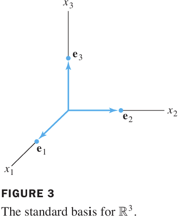
Example 5 (textbook) - The set \(\{\mathbf{e}_1,\dots,\mathbf{e}_n\}\) (columns of the \(n\times n\) identity matrix) is the standard basis for \(\mathbb{R}^n\).
they are the standard basis vectors for \(\mathbb{R}^n\) because they are linearly independent and span\(\mathbb{R}^n\) by the invertible matrix theorem (IMT).
Comments: In this specific example, the subspace \(H\) is \(\mathbb{R}^n\) itself. If a set of vectors spans all of \(\mathbb{R}^n\), it certainly spans every vector in any subset \(H \subset \mathbb{R}^n\) (because every vector in \(H\) is also in \(\mathbb{R}^n\)). However, to be a basis for a specific subspace\(H\), the vectors must satisfy the condition:
The vectors must be in\(H\) (since a basis is a set of vectors in\(H\)).
N.B. In general, for a set of \(p\) vectors \(\{v_1, \dots, v_p\}\) forming the matrix \(A = [v_1 \dots v_p]\). To prove the vectors form a basis for a subspace\(H\) (where \(H\) is not necessarily all of \(\mathbb{R}^n\)), we need to check three requirements in the definition:
Verify the vectors are in\(H\) (seems trivial, but this is often the forgotten step).
Check linear independence: Show \(Ax = 0\) has only the trivial solution.
Check that they span\(H\): Show that for every\(b \in H\), the equation \(Ax = b\) is consistent.
Example 6 (textbook) – Find a basis for the null space of the matrix
Step 1: write the solution of \(A\mathbf{x} = \mathbf{0}\) in parametric vector form (since the null space consists of all solutions to \(A\mathbf{x} = \mathbf{0}\)).
Row reduce the augmented matrix \([A \ \mathbf{0}]\) and get the equations from the reduced row echelon form,
Identify the free variables: The pivot columns are columns 1 and 3, therefore the free variables are: \(x_2, \quad x_4, \quad x_5.\) We solve for the pivot variables \(x_1\) and \(x_3\) in terms of the free variables:
Step 2: Explain why \(\{\mathbf{u}, \mathbf{v}, \mathbf{w}\}\) is a basis for \(\operatorname{Nul} A\)
The expression above shows that every vector in \(\operatorname{Nul} A\) can be written as a linear combination of \(\mathbf{u}, \mathbf{v},\) and \(\mathbf{w}\). In other words, \(\{\mathbf{u}, \mathbf{v}, \mathbf{w}\}\)spans\(\operatorname{Nul} A\).
Now we must check that these three vectors are linearly independent. Suppose
Look at entries 2, 4, and 5 of this vector equation:
Entry 2 gives \(c_1 = 0\).
Entry 4 gives \(c_2 = 0\).
Entry 5 gives \(c_3 = 0\).
Thus all coefficients must be zero, proving that \(\mathbf{u}, \mathbf{v}, \mathbf{w}\) are linearly independent.
Key Takeaway
The standard method—solving \(A\mathbf{x} = \mathbf{0}\), writing the solution in parametric form, and extracting the vectors that multiply the free variables—automatically yields a linearly independent spanning set, i.e. a basis for \(\operatorname{Nul} A\).
The number of vectors in the basis equals the number of free variables (here, 3). In general,
Nullity :=\(\text{dim}(\text{Nul } A)\)= Number of free variables.
(More will be introduced in the following section.)
Example 7 & 8 (textbook). Finding a Basis for the Column Space (less work than finding a basis for the null space)
Example 7 (A Simple Case in Reduced Row Echelon Form)
Find a basis for the column space of the matrix \(B = \begin{bmatrix} 1 & 0 & -3 & 5 & 0 \\ 0 & 1 & 2 & -1 & 0 \\ 0 & 0 & 0 & 0 & 1\\0 & 0 & 0 & 0 & 0 \end{bmatrix}\).
Sol.
Denote the columns of \(B\) by \(\mathbf{b}_1, \ldots, \mathbf{b}_5\). Observe that
Step 1: Show that the pivot columns span\(\operatorname{Col} B\)
The pivot columns of \(B\) are columns 1, 2, and 5 (since they contain the leading 1s). The fact that \(\mathbf{b}_3\) and \(\mathbf{b}_4\) are linear combinations of the pivot columns means that any combination of all five columns can be reduced to a combination of just \(\mathbf{b}_1, \mathbf{b}_2\), and \(\mathbf{b}_5\).
Let \(\mathbf{v}\) be any vector in \(\operatorname{Col} B\). Then
These starndard basis vectors are clearly linearly independent.
Conclusion: The pivot columns of \(B\) — namely \(\mathbf{b}_1, \mathbf{b}_2, \mathbf{b}_5\) — form a basis for \(\operatorname{Col} B\).
Key Takeaway for General Matrices
The matrix \(B\) in Example 7 is in reduced echelon form. For a general matrix \(A\), recall that linear dependence relations among the columns of \(A\) can be expressed as \(A\mathbf{x} = \mathbf{0}\) for some \(\mathbf{x}\). When \(A\) is row reduced to echelon form \(B\), the columns are drastically changed, but the equations
have exactly the same solution set. Therefore, the columns of\(A\)have precisely the same linear dependence relationships as the columns of\(B\).
Comment: In Example 7, matrix \(B\) is an echelon form of a certain general matrix \(A\). The pivot columns of \(B\) are columns 1, 2, 5. The corresponding columns of the original matrix\(A\)are a basis for\(\operatorname{Col} A\). (Warning: use columns from the original \(A\), not from the echelon form! The echelon form’s columns usually do not belong to \(\operatorname{Col} A\).
Because row operations preserve linear dependence relations among columns, the same relations must hold among the columns of \(A\). Hence we should have
Step 3: Argue that the pivot columns of\(A\) span \(\operatorname{Col} A\)
Since \(\mathbf{a}_3\) and \(\mathbf{a}_4\) are combinations of \(\mathbf{a}_1\) and \(\mathbf{a}_2\), any linear combination of all five columns can be rewritten as a combination of just \(\mathbf{a}_1, \mathbf{a}_2\), and \(\mathbf{a}_5\). Therefore,
Step 4: Argue that the pivot columns of\(A\) are linearly independent
Suppose there were a dependence relation among \(\mathbf{a}_1, \mathbf{a}_2\), and \(\mathbf{a}_5\). Since \(A\) and \(B\) have the same dependence relations, that same relation would hold among \(\mathbf{b}_1, \mathbf{b}_2\), and \(\mathbf{b}_5\). But \(\{\mathbf{b}_1, \mathbf{b}_2, \mathbf{b}_5\}\) is linearly independent (as shown in Example 7). Hence no such dependence relation can exist. So \(\{\mathbf{a}_1, \mathbf{a}_2, \mathbf{a}_5\}\) is linearly independent.
The pivot columns of a matrix\(A\) form a basis for \(\operatorname{Col} A\). (The proof uses the fact that row operations preserve linear dependence relations among columns.)
Interpretations:
The reasoning from Examples 7 and 8 generalizes to any matrix:
Spanning: In the reduced echelon form \(B\), every non‑pivot column is a linear combination of the pivot columns. Because row operations preserve dependence relations, the same is true for the original matrix \(A\). Hence the pivot columns of \(A\) span \(\operatorname{Col} A\).
Linear Independence: The pivot columns of \(B\) are linearly independent (they contain the identity matrix in the pivot rows). Since \(A\) and \(B\) have the same dependence relations, the pivot columns of \(A\) must also be linearly independent.
Therefore, the pivot columns of \(A\) satisfy both conditions for a basis.
N.B. 1. Use the pivot columns of\(A\)itself — not the columns of its echelon form \(B\) — for the basis of \(\operatorname{Col} A\).
N.B.2. The columns of \(B\) are often not in the column space of \(A\). (Reason: Row operations radically change the column space. While row operations preserve the linear dependence relations among columns, they do not preserve the actual column vectors themselves. Col \(A\) and Col \(B\) are generally entirely different subspaces – that’s why we must use the pivot columns of the original\(A\) for the basis.) For example, take the first pivot column of \(B\): \[ b_1 = \begin{bmatrix} 1 \\ 0 \\ 0 \\ 0 \end{bmatrix} \]Is \(b_1\) in Col \(A\)?
To be in Col \(A\), there must be scalars \(x_1, x_2, x_5\) such that \(x_1 a_1 + x_2 a_2 + x_5 a_5 = b_1\).
If we solve the first three equations, we obtain \(x_5=x_1+x_2\), \(x_1=-\frac{4}{3}x_2\), \(x_2 = \frac{3}{14}\). Plugging this into the 4th equation gives \(\frac{8}{14} \neq 0\). The system is inconsistent.
Therefore, \(b_1\) is not in Col \(A\).
Summary Table
Space
How to find a basis
\(\operatorname{Col} A\)
Take the pivot columns of the original matrix \(A\).
\(\operatorname{Nul} A\)
Solve \(A\mathbf{x} = \mathbf{0}\) and extract vectors corresponding to free variables.
Practice Problems (in‑class)
Is \(H = \left\{ \begin{bmatrix} x \\ y \\ 0 \end{bmatrix} : x,y \in \mathbb{R} \right\}\) a subspace of \(\mathbb{R}^3\)? (Hint: Verify the three conditions.)
Given \(A = \begin{bmatrix} 1 & 3 & 0 & 2 \\ 0 & 0 & 1 & -1 \\ 0 & 0 & 0 & 0 \end{bmatrix}\), determine if \(\mathbf{v} = \begin{bmatrix} 5 \\ 1 \\ -2 \\ 0 \end{bmatrix}\) is in \(\operatorname{Nul} A\). Is \(\mathbf{v}\) in \(\operatorname{Col} A\)? Justify.
True or False: The column space of an \(m\times n\) matrix is a subspace of \(\mathbb{R}^n\). Explain.
(Solutions follow at the end.)
R Supplement
library(pracma)# Example: check if vector is in Col A (by solving Ax = b)A <-matrix(c(1,-4,-3, -3,6,7, -4,-2,6), nrow=3)b <-c(3,3,-4)# Solve: consistent?aug <-cbind(A, b)rref(aug) # shows no row [0 0 0 | nonzero] -> consistent -> b in Col A
              b
[1,] 1 0 5 -4.5
[2,] 0 1 3 -2.5
[3,] 0 0 0  0.0
# Find basis for Null A of a given matrixA2 <-matrix(c(1,-2,0,2,3, 0,0,1,4,-2, 0,0,0,0,0), nrow=3, byrow=TRUE)# Null space basis via parametric form can be obtained from rrefrrefA2 <-rref(A2)# Identify free columns and construct basis vectors manually or using a function# (We'll just show the parametric vectors as in the example)u <-c(2,1,0,0,0)v <-c(-2,0,-4,1,0)w <-c(-3,0,2,0,1)# Check that A2 %*% each vector gives 0A2 %*% u
     [,1]
[1,]    0
[2,]    0
[3,]    0
A2 %*% v
     [,1]
[1,]    0
[2,]    0
[3,]    0
A2 %*% w
     [,1]
[1,]    0
[2,]    0
[3,]    0
# Basis for Col A: pivot columns of original matrixA3 <-matrix(c(2,1,-1, -4,-2,2, 2,1,-1, 0,3,0), nrow=3)(rrefA3 <-rref(A3)) # identify pivot columns (1 and 2)
\(H\) consists of all vectors of the form \((x,y,0)^T\). This is the \(xy\)-plane through the origin in \(\mathbb{R}^3\).
\(\mathbf{0} = (0,0,0)^T \in H\).
Take \(\mathbf{u}=(x_1,y_1,0)\), \(\mathbf{v}=(x_2,y_2,0)\); then \(\mathbf{u}+\mathbf{v} = (x_1+x_2, y_1+y_2, 0)\in H\).
For scalar \(c\), \(c\mathbf{u} = (cx_1, cy_1, 0)\in H\).
All three properties hold, so \(H\) is a subspace.
Given \(A = \begin{bmatrix} 2 & -4 & 2 & 0 \\ 1 & -2 & 1 & 3 \\ -1 & 2 & -1 & 0 \end{bmatrix}\).
part a. Row reduce \(A\) to echelon form: \[\begin{bmatrix} 2 & -4 & 2 & 0 \\ 1 & -2 & 1 & 3 \\ -1 & 2 & -1 & 0 \end{bmatrix}
\xrightarrow{\text{swap}} \text{ or directly...}\] For brevity: after reduction we get \[\begin{bmatrix} 1 & -2 & 1 & 0 \\ 0 & 0 & 0 & 1 \\ 0 & 0 & 0 & 0 \end{bmatrix} \text{ or row equivalent.}\] Pivot columns: column 1 and column 4.
So according to theorem 13, the basis for \(\operatorname{Col} A\): the first and fourth columns of the original \(A\), i.e., \(\begin{bmatrix} 2 \\ 1 \\ -1 \end{bmatrix}\) and \(\begin{bmatrix} 0 \\ 3 \\ 0 \end{bmatrix}\).
part b. For \(\operatorname{Nul} A\), solve \(A\mathbf{x}=\mathbf{0}\). The reduced echelon form of \(A\) is \[\begin{bmatrix} 1 & -2 & 1 & 0 \\ 0 & 0 & 0 & 1 \\ 0 & 0 & 0 & 0 \end{bmatrix}.\] So \(x_1 - 2x_2 + x_3 = 0\) and \(x_4 = 0\). Free variables: \(x_2\), \(x_3\). General solution: \[x_1 = 2x_2 - x_3,\quad x_4 = 0.\] In vector form: \[\mathbf{x} = \begin{bmatrix} 2x_2 - x_3 \\ x_2 \\ x_3 \\ 0 \end{bmatrix} = x_2\begin{bmatrix} 2 \\ 1 \\ 0 \\ 0 \end{bmatrix} + x_3\begin{bmatrix} -1 \\ 0 \\ 1 \\ 0 \end{bmatrix}.\] The two vectors \(\begin{bmatrix} 2 \\ 1 \\ 0 \\ 0 \end{bmatrix}\) and \(\begin{bmatrix} -1 \\ 0 \\ 1 \\ 0 \end{bmatrix}\) are linearly independent and span \(\operatorname{Nul} A\), so they form a basis.
Check if \(\mathbf{v} = (5,1,-2,0)^T \in \operatorname{Nul} A\): Compute \(A\mathbf{v} = \begin{bmatrix} 1(5)+3(1)+0(-2)+2(0) \\ 0+0+1(-2)+(-1)(0) \\ 0 \end{bmatrix} = \begin{bmatrix} 8 \\ -2 \\ 0 \end{bmatrix} \neq \mathbf{0}\), so not in \(\operatorname{Nul} A\).
Is \(\mathbf{v}\) in \(\operatorname{Col} A\)? Since \(\operatorname{Col} A\) is a subspace of \(\mathbb{R}^3\). However, we need to check if \(\mathbf{v}\) (which is \(4\times 1\)) is in \(\operatorname{Col} A\). Note that \(\operatorname{Col} A\) consists of vectors in \(\mathbb{R}^3\), while \(\mathbf{v}\) is a vector in \(\mathbb{R}^4\). So \(\mathbf{v}\) cannot be in \(\operatorname{Col} A\) because the dimensions do not match. Therefore, the answer is no.
False. The column space of an \(m\times n\) matrix \(A\) is a set of linear combinations of its columns, each of which is a vector in \(\mathbb{R}^m\) (because \(A\) has \(m\) rows). Thus \(\operatorname{Col} A\) is a subspace of \(\mathbb{R}^m\), not \(\mathbb{R}^n\). (The null space is the one that lives in \(\mathbb{R}^n\).)
Summary
A subspace is a set that contains the zero vector and is closed under addition and scalar multiplication.
The span of any set of vectors is a subspace.
\(\operatorname{Col} A\) is the span of the columns (subset of \(\mathbb{R}^m\)); \(\operatorname{Nul} A\) is the solution set of \(A\mathbf{x}=\mathbf{0}\) (subset of \(\mathbb{R}^n\)).
The pivot columns of \(A\) form a basis for \(\operatorname{Col} A\).
A basis for \(\operatorname{Nul} A\) is obtained from the parametric vector form of the general solution to \(A\mathbf{x}=\mathbf{0}\).
Next week we will study dimension (the number of vectors in a basis) and rank, expanding the Invertible Matrix Theorem.
Section 2.9 Dimension and Rank
Learning Objectives
After this lecture you will be able to:
Explain the concept of coordinates relative to a basis and compute coordinate vectors.
Define the dimension of a subspace and find the dimension of common subspaces.
Define the rank of a matrix and state the Rank Theorem.
Find the rank of a matrix by counting pivot columns.
Use the Rank Theorem to relate the dimension of the column space and the null space.
Extend the Invertible Matrix Theorem with statements about basis, dimension, and rank.
Apply the Basis Theorem to automatically recognize a basis from a set of vectors with the right number and appropriate property (independence or spanning).
Coordinate Systems
Definition
If \(\mathcal B = \{\mathbf{b}_1,\dots,\mathbf{b}_p\}\) is a basis for a subspace \(H\), then each \(\mathbf{x} \in H\) can be written uniquely as a linear combination \[\mathbf{x} = c_1\mathbf{b}_1 + \cdots + c_p\mathbf{b}_p.\] The weights \(c_1,\dots,c_p\) are the coordinatesof\(\mathbf{x}\)relative to the basis\(\mathcal B\). The vector \[[\mathbf{x}]_{\mathcal B} = \begin{bmatrix} c_1 \\ \vdots \\ c_p \end{bmatrix} \in \mathbb{R}^p\] is the coordinate vector of \(\mathbf{x}\) (relative to \(\mathcal B\)) or the \(\mathcal B\)‑coordinate vector of \(\mathbf{x}\) .
Example 1 (textbook). Let \(\mathbf{v}_1 = \begin{bmatrix} 3 \\ 6 \\ 2 \end{bmatrix},\,
\mathbf{v}_2 = \begin{bmatrix} -1 \\ 0 \\ 1 \end{bmatrix},\,
\mathbf{x} = \begin{bmatrix} 3 \\ 12 \\ 7 \end{bmatrix}\), and \(\mathcal B = \{\mathbf{v}_1,\mathbf{v}_2\}\). \(\mathcal B\) is a basis for \(H = \operatorname{Span}\{\mathbf{v}_1,\mathbf{v}_2\}\) because \(\mathbf{v}_1,\mathbf{v}_2\) are linearly independent (not multiples).
Find the \(\mathcal B\)‑coordinates of \(\mathbf{x}\).
Set up \(c_1\mathbf{v}_1 + c_2\mathbf{v}_2 = \mathbf{x}\):
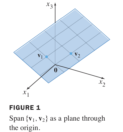
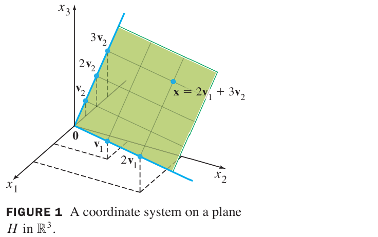
Geometrically, the basis vectors \(\mathcal B\) determine a “coordinate system/grid” on the plane \(H\).
Supplementary Comments on The Coordinate System and Figure 1:
Although \(H\) is a plane embedded in \(\mathbb{R}^3\), the basis \(\mathcal{B} = \{\mathbf{v}_1, \mathbf{v}_2\}\) gives it a two‑dimensional coordinate system that makes \(H\) behave exactly like \(\mathbb{R}^2\).
How the grid works:
The grid on \(H\) (Figure 1) is formed by taking all linear combinations \[c_1\mathbf{v}_1 + c_2\mathbf{v}_2\] where \(c_1\) and \(c_2\) range over integers (or real numbers). This is analogous to the standard grid in the \(xy\)-plane:
The lines parallel to \(\mathbf{v}_1\) correspond to holding \(c_2\) constant and varying \(c_1\).
The lines parallel to \(\mathbf{v}_2\) correspond to holding \(c_1\) constant and varying \(c_2\).
Just as every point in \(\mathbb{R}^2\) has a unique address \((c_1, c_2)\), every point in \(H\) has a unique coordinate vector\([\mathbf{x}]_{\mathcal{B}} = \begin{bmatrix} c_1 \\ c_2 \end{bmatrix}\).
In this example, \([\mathbf{x}]_{\mathcal{B}} = \begin{bmatrix} 2 \\ 3 \end{bmatrix}\). Geometrically, this means that to reach \(\mathbf{x}\) starting from the origin in \(H\), you move: \(2\) units along \(\mathbf{v}_1\) (i.e., \(2\mathbf{v}_1\)), and then \(3\) units along \(\mathbf{v}_2\) (i.e., \(3\mathbf{v}_2\)).
Why this is an isomorphism:
The mapping \[\mathbf{x} \longmapsto [\mathbf{x}]_{\mathcal{B}}\] is a one‑to‑one correspondence between \(H\) and \(\mathbb{R}^2\). Moreover, it preserves linear combinations: \[[\mathbf{u} + \mathbf{v}]_{\mathcal{B}} = [\mathbf{u}]_{\mathcal{B}} + [\mathbf{v}]_{\mathcal{B}}, \qquad
[c\mathbf{u}]_{\mathcal{B}} = c[\mathbf{u}]_{\mathcal{B}}.\]
This preservation property means that \(H\) is isomorphic to \(\mathbb{R}^2\) — algebraically, they are indistinguishable. Even though the vectors in \(H\) have three entries, their coordinate vectors have only two entries, and all calculations (addition, scalar multiplication, linear dependence) can be carried out entirely in \(\mathbb{R}^2\) using the coordinates.
In short: The grid on \(H\) turns the plane into a perfect copy of \(\mathbb{R}^2\), with \(\mathbf{v}_1\) and \(\mathbf{v}_2\) playing the roles of the standard coordinate axes.
Dimension of a Subspace
Definition
The dimension of a nonzero subspace \(H\), written \(\dim H\), is the number of vectors in any basis for \(H\).
By convention, \(\dim\{\mathbf{0}\} = 0\).
\(\dim \mathbb{R}^n = n\) (the standard basis has \(n\) vectors).
A line through the origin has dimension 1.
A plane through the origin has dimension 2.
The dimension is well‑defined because every basis for a given subspace has the same number of vectors (this is proved in Section 4.5, but we can rely on the concept now).
Rank of a Matrix
Definition
The rank of a matrix \(A\), written \(\operatorname{rank} A\), is the dimension of the column space of \(A\):
\[\operatorname{rank} A = \dim \operatorname{Col} A.\]
Since the pivot columns of \(A\) form a basis for \(\operatorname{Col} A\), the rank equals the number of pivot columns in \(A\).
There are three pivot columns (1, 2, 4), so \(\operatorname{rank} A = 3\).
Theorem 14 - The Rank Theorem
Pivot columns correspond to basic variables, while non‑pivot columns correspond to free variables in solving \(A\mathbf{x} = \mathbf{0}\). Since every column is either a pivot column or a non‑pivot column, we have the elegant relationship:
Theorem 14 (Rank-Nullity Theorem).
If \(A\) is an \(m \times n\) matrix, then \[\operatorname{rank} A + \dim \operatorname{Nul} A = n.\]
Note:\(n\) is the number of columns. \(\dim \operatorname{Nul} A\) is called the nullity of \(A\), though we will not often use this term.
Thus, knowing the rank immediately gives the dimension of the null space, and vice versa.
Example. For the \(A\) in Example 3, \(n = 5\), \(\operatorname{rank} A = 3\), so \(\dim \operatorname{Nul} A = 2\). Indeed, there are 5 columns and 3 pivot columns → 2 free variables.
Theorem 15 - The Basis Theorem
The following theorem helps determine when a set of vectors forms a basis without checking both independence and spanning.
Theorem 15 (The Basis Theorem).
Let \(H\) be a \(p\)‑dimensional subspace of \(\mathbb{R}^n\).
Any linearly independent set of exactly \(p\) vectors in \(H\) is a basis for \(H\).
Any set of \(p\) vectors that spans \(H\) is a basis for \(H\).
Core Intuition: In a \(p\)‑dimensional subspace, if you grab the “right” number of vectors—exactly \(p\) of them—then having one basis-property automatically guarantees the other. You don’t need to check both spanning and linear independence.
Interpretations of Theorem 15
Interpretation of Statement 1 (Independence\(\Rightarrow\)Spanning):
In a \(p\)-dimensional space, the maximum size of a linearly independent set is \(p\). If you already have \(p\) independent vectors, the space is “full” of independent directions. There is no room left to add another independent vector, meaning these \(p\) vectors must reach every corner of \(H\). Thus, they automatically span \(H\).
Interpretation of Statement 2 (Spanning\(\Rightarrow\)Independence):
If \(p\) vectors are enough to cover the entire subspace \(H\) by spanning it, then none of them can be redundant. If one were a linear combination of the others, you could throw it away and still span \(H\) with only \(p-1\) vectors—which is impossible in a \(p\)-dimensional space. Hence, they must be linearly independent.
Example. Is \(\left\{ \begin{bmatrix} 1 \\ 0 \\ 2 \end{bmatrix}, \begin{bmatrix} 0 \\ 1 \\ -1 \end{bmatrix} \right\}\) a basis for \(\mathbb{R}^3\)?
Here, \(H = \mathbb{R}^3\), so \(p = n = 3\). Since we only have 2 vectors (and \(2 \neq p\)), the theorem does not apply to make them a basis. They are independent, but they fall short of spanning the 3D space—they only span a 2‑dimensional plane.
Caveat I:Distinguishing\(p\)vs.\(n\)
Do not confuse the subspace dimension\(p\) with the ambient dimension \(n\). The theorem works for any subspace, whether \(p = n\) or \(p < n\).
\(n\) = the number of coordinates in each vector (the size of the big space \(\mathbb{R}^n\)).
\(p\) = the dimension of your specific subspace \(H\) (the number of vectors in a basis for \(H\)).
Example of\(p \leq n\):
Let the ambient space be \(\mathbb{R}^3\) (\(n = 3\)).
Let \(H\) be a plane through the origin, such as \[ H = \text{span}\left\{\begin{bmatrix} 1 \\ 0 \\ 0 \end{bmatrix}, \begin{bmatrix} 0 \\ 1 \\ 0 \end{bmatrix}\right\}. \] This plane has dimension \(p = 2\), even though \(n = 3\).
Now, apply Theorem 15 to this \(H\):
Any 2linearly independent vectors inside this plane (e.g., \(\begin{bmatrix} 1 \\ 1 \\ 0 \end{bmatrix}\) and \(\begin{bmatrix} 1 \\ -1 \\ 0 \end{bmatrix}\)) form a basis for the plane.
Notice that these 2 vectors do not span all of \(\mathbb{R}^3\) (you need 3 vectors for that), but they do span this specific 2D subspace \(H\). The theorem holds perfectly because we are only concerned with \(p=2\), not \(n=3\).
Caveat II: The Vectors MUST Belong to \(H\) (The ” in \(H\) ” Rule)
This is the most common pitfall. Having exactly \(p\) vectors is necessary to use the shortcut, but it is not sufficient on its own. Before applying Theorem 15, you must verify that the vectors actually live inside the subspace \(H\). If they are outside \(H\), the theorem is invalid.
Example of Caveat II (Failure Case):
Using the same \(xy\)-plane \(H\) as in caveat I (where the third coordinate must be \(0\)), consider: \[ v_1 = \begin{bmatrix} 1 \\ 0 \\ 2 \end{bmatrix}, \quad v_2 = \begin{bmatrix} 0 \\ 1 \\ -1 \end{bmatrix} \]
We have exactly \(p=2\) vectors. However, \(v_1\) has a third coordinate of \(2\), and \(v_2\) has a third coordinate of \(-1\). Neither vector is in\(H\).
Conclusion: They cannot be a basis for \(H\). The theorem does not apply here.
Example of Caveat II (Success Case):
Still using the same \(xy\)-plane \(H\), consider: \[ w_1 = \begin{bmatrix} 1 \\ 2 \\ 0 \end{bmatrix}, \quad w_2 = \begin{bmatrix} -3 \\ 4 \\ 0 \end{bmatrix} \]
We have exactly \(p=2\) vectors. Both vectors are in\(H\) (third coordinate is \(0\)).
They are linearly independent (neither is a scalar multiple of the other). By Theorem 15 Statement 1, since we have \(p=2\) independent vectors inside\(H\), they automatically span \(H\). Therefore, \(\{w_1, w_2\}\) is a basis for \(H\).
Step-by-Step Checklist
When asked if a set of vectors forms a basis for a subspace \(H\):
Identify\(p\): What is the dimension of \(H\)? (e.g., Is it a plane? \(p=2\). Is it \(\mathbb{R}^3\)? \(p=3\). Is it a line? \(p=1\).)
Count the vectors: Do you have exactly \(p\) vectors?
If NO: Stop. They cannot be a basis (too few can’t span; too many can’t be independent).
If YES: Proceed to Step 3.
Check membership: Are all the vectors actually contained in \(H\)?
If NO: Stop. They cannot be a basis.
If YES: Proceed to Step 4.
Apply Theorem 15: Now that you have the right number and they are in the right place, check only one of the two properties (whichever is easier):
Check if they are linearly independent (if yes, they span \(H\)).
OR check if they span \(H\) (if yes, they are independent).
Either way, if the single check passes, they are a basis for \(H\).
Extensions to the Invertible Matrix Theorem
The concepts of dimension and rank add more equivalent statements to the IMT:
Theorem (IMT continued).
Let \(A\) be an \(n\times n\) matrix. The following are equivalent to \(A\) being invertible.
The columns of \(A\) form a basis of \(\mathbb{R}^n\).
\(\operatorname{Col} A = \mathbb{R}^n\).
\(\dim \operatorname{Col} A = n\) (i.e., \(\operatorname{rank} A = n\)).
\(\operatorname{rank} A = n\).
\(\operatorname{Nul} A = \{\mathbf{0}\}\).
\(\dim \operatorname{Nul} A = 0\).
All of these follow from earlier parts of the IMT and the Rank Theorem.
Proof Strategy.
The proof proceeds in two logical parts:
Show that statement (m) is equivalent to previously known statements (e) and (h) (linear independence and spanning).
Establish a chain of implications: \[ (g) \Rightarrow (n) \Rightarrow (o) \Rightarrow (p) \Rightarrow (r) \Rightarrow (q) \Rightarrow (d) \] Since statements (g) and (d) are already known to be equivalent to invertibility, this chain proves that all new statements are also equivalent to invertibility.
Proof.
Part 1: Statement (m) is Equivalent to Invertibility.
Recall the definition of a basis: A basis is a set of vectors that is linearly independent and spans the space.
Statement (e) from the original IMT says: The columns of\(A\) form a linearly independent set.
Statement (h) from the original IMT says: The columns of\(A\) span \(\mathbb{R}^n\).
and both (e) and (h) are already known to be equivalent to invertibility, it follows immediately that (m) is also equivalent to invertibility.
Part 2: The Chain of Implications \[ (g) \Rightarrow (n) \Rightarrow (o) \Rightarrow (p) \Rightarrow (r) \Rightarrow (q) \Rightarrow (d) \]
Step 1: (g)\(\Rightarrow\) (n)
Statement (g): The equation\(A\mathbf{x} = \mathbf{b}\) has at least one solution for every \(\mathbf{b} \in \mathbb{R}^n\).
Recall that the column space of \(A\), denoted \(\operatorname{Col} A\), is exactly the set of all vectors \(\mathbf{b}\) for which the equation \(A\mathbf{x} = \mathbf{b}\) is consistent (i.e., has at least one solution).
If (g) holds, then every vector \(\mathbf{b} \in \mathbb{R}^n\) is in the column space of \(A\). Therefore, \(\operatorname{Col} A\) contains all of \(\mathbb{R}^n\).
Since \(\operatorname{Col} A\) is a subspace of \(\mathbb{R}^n\), it cannot be larger than \(\mathbb{R}^n\). So we must have: \[ \operatorname{Col} A = \mathbb{R}^n. \]
Step 2: (n)\(\Rightarrow\) (o)
The dimension of \(\mathbb{R}^n\) is \(n\).
Therefore, if \(\operatorname{Col} A = \mathbb{R}^n\), then its dimension is \(n\): \[ \dim \operatorname{Col} A = n. \]
Step 3: (o) \(\Rightarrow\) (p)
By definition, the rank of a matrix \(A\) is the dimension of its column space: \[ \operatorname{rank} A = \dim \operatorname{Col} A. \]
Therefore, if \(\dim \operatorname{Col} A = n\), then: \[ \operatorname{rank} A = n. \]
Step 4: (p) \(\Rightarrow\) (r)
We use the Rank Theorem (also known as the Rank-Nullity Theorem): \[ \operatorname{rank} A + \dim \operatorname{Nul} A = n \] where \(n\) is the number of columns of \(A\).
Substituting \(\operatorname{rank} A = n\) into the Rank Theorem gives: \[ n + \dim \operatorname{Nul} A = n \quad \Rightarrow \quad \dim \operatorname{Nul} A = 0. \]
Step 5: (r)\(\Rightarrow\) (q)
The null space \(\operatorname{Nul} A\) is a subspace. The only subspace of \(\mathbb{R}^n\) that has dimension \(0\) is the trivial subspace containing only the zero vector. Therefore: \[ \operatorname{Nul} A = \{\mathbf{0}\}. \]
Step 6: (q)\(\Rightarrow\) (d)
By definition, the null space of \(A\) is the set of all solutions to the homogeneous equation \(A\mathbf{x} = \mathbf{0}\).
If the null space contains only the zero vector, then the only solution to \(A\mathbf{x} = \mathbf{0}\) is the trivial solution \(\mathbf{x} = \mathbf{0}\). This is exactly statement (d): The equation\(A\mathbf{x} = \mathbf{0}\) has only the trivial solution.
Key Takeaway
The extended Invertible Matrix Theorem now provides a comprehensive set of criteria for invertibility, spanning multiple areas: row operations, linear systems, linear independence, spanning, basis, column space, null space, rank, and dimension. This unified framework is one of the most powerful tools in linear algebra, allowing us to translate between algebraic, geometric, and computational perspectives.
Example: A \(4\times 4\) matrix has \(\operatorname{rank} A = 4\). Then by IMT(o) it is invertible; consequently \(\dim \operatorname{Nul} A = 0\) and \(A\mathbf{x}=\mathbf{0}\) has only the trivial solution.
Practice Problems (in‑class)
Let \(\mathcal B = \left\{ \begin{bmatrix} 1 \\ -2 \end{bmatrix}, \begin{bmatrix} -2 \\ 5 \end{bmatrix} \right\}\) be a basis for \(\mathbb{R}^2\). If \([\mathbf{x}]_\mathcal B = \begin{bmatrix} 3 \\ -1 \end{bmatrix}\), find \(\mathbf{x}\).
If \(A\) is a \(5\times 7\) matrix with rank 4, what is \(\dim \operatorname{Nul} A\)? Can the columns of \(A\) span \(\mathbb{R}^5\)? Explain.
Is the set \(\left\{ \begin{bmatrix} 1 \\ 2 \\ 0 \end{bmatrix}, \begin{bmatrix} 0 \\ 1 \\ 2 \end{bmatrix}, \begin{bmatrix} 1 \\ 1 \\ 0 \end{bmatrix} \right\}\) a basis for \(\mathbb{R}^3\)? Use the Basis Theorem or the IMT to justify.
True or False: If \(A\) is a \(7\times 9\) matrix and \(\dim \operatorname{Nul} A = 3\), then the columns of \(A\) are linearly independent. Justify.
(Solutions at the end.)
R Supplement
library(pracma)# Coordinate vector example: solve linear combinationB <-matrix(c(1,-2, -2,5), nrow=2) # columns are basis vectorscoords <-c(3, -1)x <- B %*% coordsx # this is x
     [,1]
[1,]    5
[2,]  -11
# Rank and nullityA <-matrix(c(1,2,-1, -1,-1,0, 2,5,-3, 0,1,-1), nrow=3, byrow=TRUE)# Row reduce to echelonrrefA <-rref(A)rrefA
# Verify null space dimension: solve Ax=0, count free variables# Not automatically, but we can check: The rref shows pivot columns.
Comments: To find the rank, the number of pivot columns and the number of non-zero rows are all equal. That is, the rank of a matrix is also the dimension of its row space (the maximum number of linearly independent rows). This is because,
in any Row Echelon Form, these two quantities are physically the same number because of how the matrix is structured:
Every non-zero row has exactly one leading entry (pivot).
Every pivot sits in a unique column (no two pivots share the same column).
Because of this one-to-one correspondence, the count of non-zero rows and the count of pivot columns are literally the exact same number when you look at the matrix. Therefore,
Rank = Number of non-zero rows =Number of pivot columns.
Part 1: \(A\) is \(5\times 7\), so \(n=7\) columns. \(\operatorname{rank} A = 4\), thus \(\dim \operatorname{Nul} A = 7 - 4 = 3\).
Part 2: No, they cannot. Here is the reasoning (Be careful, IMT is NOT applicable here.):
The columns of \(A\) live in \(\mathbb{R}^5\) because \(A\) has \(5\) rows.
By definition, the span of the columns of \(A\) is exactly the column space of \(A\), denoted \(\operatorname{Col} A\). By definition of rank, the dimension of the column space equals the rank: \[ \dim(\operatorname{Col} A) = \operatorname{rank} A = 4 \]
The column space \(\operatorname{Col} A\) is a subspace of \(\mathbb{R}^5\). Since \(\dim(\operatorname{Col} A) = 4\) is strictly less than \(\dim(\mathbb{R}^5) = 5\), the column space cannot possibly be the entire space \(\mathbb{R}^5\).
So, since the span of the columns is only a 4-dimensional subspace inside a 5-dimensional space, the columns fail to span \(\mathbb{R}^5\).
N.B. General Rule for Spanning\(\mathbb{R}^m\):
For an \(m \times n\) matrix \(A\), the columns of \(A\) span \(\mathbb{R}^m\)if and only if\(\operatorname{rank} A = m\).
(This follows directly from the definition of rank = dimension of the column space, and it applies to all matrices, square or rectangular.)
In this specific problem, \(m = 5\) and \(\operatorname{rank} A = 4 \neq 5\), so the columns do not span \(\mathbb{R}^5\).
The three vectors are in \(\mathbb{R}^3\). By the Basis Theorem, for a 3‑dimensional space, if they are linearly independent they form a basis. Check independence: form matrix with vectors as columns and row reduce: \[\begin{bmatrix} 1 & 0 & 1 \\ 2 & 1 & 1 \\ 0 & 2 & 0 \end{bmatrix}
\sim
\begin{bmatrix} 1 & 0 & 1 \\ 0 & 1 & -1 \\ 0 & 2 & 0 \end{bmatrix}
\sim
\begin{bmatrix} 1 & 0 & 1 \\ 0 & 1 & -1 \\ 0 & 0 & 2 \end{bmatrix}.\] Three pivots → columns are linearly independent. Since there are 3 vectors and \(\dim \mathbb{R}^3 = 3\), they automatically form a basis (Basis Theorem). So yes, they are a basis.
False.\(A\) is \(7\times 9\) (\(n=9\) columns). \(\dim \operatorname{Nul} A = 3\) means null space dimension is 3. By Rank Theorem, \(\operatorname{rank} A = 9 - 3 = 6\). The columns are linearly independent only if \(\operatorname{rank} A = 9\). However, here rank is 6, which means there are 3 columns that are combinations of the pivots → columns are linearly dependent.
N.B.General Rule forthe Linear Independence of Columns:
For any \(m \times n\) matrix, the columns are linearly independent if and only if
\[\operatorname{rank} A = n\]
In this question, \(\operatorname{rank} A = 6\), but the number of columns is \(n = 9\).
A Summary of The Rules as Two Direct Corollaries of the Basis Theorem (Theorem 15).
Rule 1: Columns span\(\mathbb{R}^m\)\(\Longleftrightarrow\)\(\operatorname{rank} A = m\)
Proof (Optional):
(\(\Rightarrow\)) If the columns of \(A\) span \(\mathbb{R}^m\), then by definition of the column space of \(A\), \(\operatorname{Col} A\) equals the entire space \(\mathbb{R}^m\). Therefore: \[ \operatorname{rank} A = \dim(\operatorname{Col} A) = \dim(\mathbb{R}^m) = m \]
(\(\Leftarrow\)) If \(\operatorname{rank} A = m\), then there are exactly \(m\) pivot columns in \(A\).
These \(m\) pivot columns are linearly independent (by the definition of pivot columns).
These \(m\) pivot columns live in \(\mathbb{R}^m\) (since \(A\) has \(m\) rows).
Now apply Theorem 15 (Statement 1) with \(H = \mathbb{R}^m\) and \(p = m\):
*“Any linearly independent set of exactly* \(p\) vectors in a \(p\)-dimensional space \(H\) is a basis for \(H\).”
Here, \(H = \mathbb{R}^m\) is \(m\)-dimensional, and we have exactly \(m\) independent pivot columns. Therefore, these pivot columns form a basis for \(\mathbb{R}^m\), meaning they span \(\mathbb{R}^m\).
Since the original set of all columns of \(A\) contains these pivot columns, the original columns also span \(\mathbb{R}^m\).
Conclusion:\(\text{Columns span } \mathbb{R}^m \iff \operatorname{rank} A = m\).
Rule 2: Columns are linearly independent\(\Longleftrightarrow\)\(\operatorname{rank} A = n\)
Proof (Optional):
Let the \(n\) columns of \(A\) be \(\mathbf{a}_1, \mathbf{a}_2, \dots, \mathbf{a}_n\). Let their span be the column space \(H = \operatorname{Col} A\). We know: \[ \dim(H) = \dim(\operatorname{Col} A) = \operatorname{rank} A \]
(\(\Rightarrow\)) If the \(n\) columns are linearly independent, then by definition they form a basis for their own span, which is \(H\). A basis for \(H\) must contain exactly \(\dim(H)\) vectors. Therefore: \[ n = \dim(H) = \operatorname{rank} A \]
(\(\Leftarrow\)) If \(\operatorname{rank} A = n\), then \(\dim(H) = n\).
We know that the \(n\) columns span\(H\) (by the very definition of column space).
Now apply Theorem 15 (Statement 2) with \(H = \operatorname{Col} A\) and \(p = n\):
*“Any set of exactly* \(p\) vectors that spans a \(p\)-dimensional space \(H\) is a basis for \(H\).”
Here, \(H\) is \(n\)-dimensional, and we have exactly \(n\) vectors (the columns) that span \(H\). Therefore, these \(n\) columns form a basis for \(H\), meaning they are linearly independent.
Conclusion:\(\text{Columns are linearly independent} \iff \operatorname{rank} A = n\).
Here is a Summary Table:
Let \(A\) be an \(m\times n\) matrix, then \(\operatorname{Col}A\subseteq \mathbb R^m\) and \(\operatorname{rank}A=\dim(\operatorname{Col}A)\).
What are we checking?
The Exact Criterion
How Theorem 15 Proves It
Span\(\mathbb{R}^m\)
\(\operatorname{rank} A = m\)
If rank = \(m\), the \(m\) pivot columns are \(m\) independent vectors in \(\mathbb{R}^m\). By Theorem 15 (Statement 1), they form a basis, so they span \(\mathbb{R}^m\).
Linearly Independent
\(\operatorname{rank} A = n\)
If rank = \(n\), the column space \(H\) has dimension \(n\). The \(n\) columns span \(H\). By Theorem 15 (Statement 2), they form a basis for \(H\), so they are independent.
Further Notes:
The two conditions can both hold only when \(m=n\) and \(A\) is invertible. Otherwise:
If \(\operatorname{rank}A=m\), the columns span \(\mathbb R^m\), but they may not be independent if \(n>m\).
If \(\operatorname{rank}A=n\), the columns are independent, but they may not span \(\mathbb R^m\) if \(m>n\).
Summary
A basis provides a coordinate system on a subspace; coordinates are the unique weights in a linear combination.
The dimension of a subspace is the number of vectors in any basis.
The rank of a matrix is the dimension of its column space; it equals the number of pivot columns.
The Rank Theorem: \(\operatorname{rank} A + \dim \operatorname{Nul} A = \text{number of columns}\).
The Basis Theorem: in a \(p\)‑dimensional space, \(p\) linearly independent vectors automatically form a basis; \(p\) spanning vectors also form a basis.
The Invertible Matrix Theorem now includes statements about rank, column space being \(\mathbb{R}^n\), and zero null space.
These concepts unify the understanding of linear systems, subspaces, and matrix invertibility.
These notes follow Chapter 2 of Lay, Lay & McDonald, “Linear Algebra and its Applications”, 5th edition.