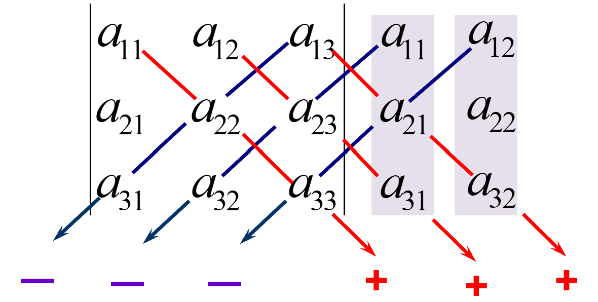
For \(n \ge 2\), the determinant of an \(n\times n\) matrix \(A = [a_{ij}]\) is defined by cofactor expansion across the first row: \[\begin{align}\det A &= a_{11}\det A_{11} - a_{12}\det A_{12} + \cdots + (-1)^{1+n}a_{1n}\det A_{1n}\\
&= \sum_{j=1}^{n} (-1)^{1+j} a_{1j} \det A_{1j}\end{align}.\]
The \((i,j)\)-cofactor of \(A\) is
\[C_{ij} = (-1)^{i+j} \det A_{ij}.\]
With this notation, the first‑row expansion becomes
\[\det A = a_{11}C_{11} + a_{12}C_{12} + \cdots + a_{1n}C_{1n}.\]
N.B. If a matrix has many zeros, choose the row or column with the most zeros for the cofactor expansion. N.B. If an entire row or column consists of zeros, the determinant is zero.
If \(A\) is a triangular matrix (upper or lower), then \(\det A\) is the product of the entries on its main diagonal.
Numerical Note
A cofactor expansion requires roughly \(n!\) multiplications. For \(n=25\), this is about \(1.5\times10^{25}\) operations – impossible even on the fastest computers. Later we will learn how row reduction reduces this to about \(2n^3/3\) operations, making determinant calculation feasible for large matrices.
Practice Problems
Compute the determinant of \(\begin{bmatrix} 2 & 3 \\ 1 & 4 \end{bmatrix}\) using the \(2\times2\) formula.
Use a cofactor expansion across the first row to compute \(\det A\) for
\(B\) is lower triangular. Its determinant is the product of the diagonal entries: \((-2)\cdot3\cdot(-4)\cdot2 = 48\).
Compute determinant. Row reduce to echelon form or use cofactor expansion. Quick row reduction: \[\begin{bmatrix}1&2&3\\4&5&6\\7&8&9\end{bmatrix}
\xrightarrow{R2-4R1,\; R3-7R1}
\begin{bmatrix}1&2&3\\0&-3&-6\\0&-6&-12\end{bmatrix}
\xrightarrow{R3-2R2}
\begin{bmatrix}1&2&3\\0&-3&-6\\0&0&0\end{bmatrix}.\] Upper triangular form has a zero on the diagonal, so determinant is \(0\). Therefore the matrix is not invertible.
Summary
The determinant is a scalar value defined recursively via cofactor expansion.
The expansion can be taken along any row or down any column; signs follow a checkerboard pattern.
The determinant of a triangular matrix equals the product of its diagonal entries.
A matrix is invertible if and only if its determinant is nonzero (a fact used heavily later).
For large matrices, row reduction is far more efficient than direct cofactor expansion.
Section 3.2 Properties of Determinants
Learning Objectives
After this lecture you will be able to:
Explain how elementary row operations affect the determinant of a matrix.
Compute determinants efficiently using row reduction to triangular form.
State the invertibility condition in terms of determinants: a square matrix is invertible iff its determinant is nonzero.
Prove that \(\det A^T = \det A\) and that column operations act on determinants in the same way as row operations.
Use the multiplicative property \(\det(AB) = \det A \det B\) to calculate determinants of products and inverses.
Recognize that the determinant is a linear function of each column when other columns are fixed.
Theorem 3 - How Row Operations Affect Determinants
The key to efficient determinant computation is knowing how elementary row operations change the determinant.
Theorem 3 (Row Operations).
Let \(A\) be a square matrix.
If a multiple of one row is added to another row to produce \(B\), then \(\det B = \det A\).
If two rows are interchanged to produce \(B\), then \(\det B = -\det A\).
If one row is multiplied by \(k\) to produce \(B\), then \(\det B = k\cdot\det A\).
These properties correspond exactly to the effect of elementary matrices:
A row replacement matrix (add a multiple of one row to another) has determinant 1.
An interchange matrix has determinant \(-1\).
A scale matrix (multiply a row by \(k\)) has determinant \(k\).
Thus for any elementary matrix \(E\), \(\det(EA) = (\det E)(\det A)\).
N.B.Scaling and scalar multiplication are different: For any \(n \times n\) matrix \(A\) and any scalar \(k\),
\[\det(kA) = k^n \det A.\]
That is, multiplying every entry of a matrix by \(k\) multiplies the determinant by \(k^n\), where \(n\) is the size of the matrix.
If \(A = \begin{bmatrix} a_{ij} \end{bmatrix}_{3 \times 3}\), then
In general, for an \(n \times n\) matrix, the factor \(k\) can be factored out of each of the \(n\) rows (or columns), giving \(k^n\).
Computing Determinants by Row Reduction
The idea: row reduce the matrix to an upper triangular form U using only row replacements and row interchanges (no scaling until the end, if needed). Then
\[\det A = (-1)^r \cdot (\text{product of the diagonal entries of } U),\]
where \(r\) is the number of row interchanges performed.
Comments: Although the echelon form \(U\) described above is not unique (because it is not completely row reduced), and the pivots are not unique, the product of the pivots is unique, except for a possible minus sign. In summary,
If \(A\) is an \(n \times n\) matrix, and we reduce it to an upper triangular matrix \(U\) using row operations, then
\[\det A =
\begin{cases}
(-1)^r \cdot \left( \text{product of pivots in } U \right) & \text{if } A \text{ is invertible}, \\[6pt]
0 & \text{if } A \text{ is not invertible}.
\end{cases}\]
Here, \(r\) is the total number of row interchanges performed during the reduction.
Theorem 4 - Determinant and Invertibility
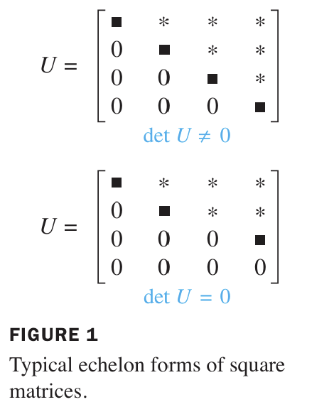
From the row reduction process, we see that a square matrix \(A\) can be reduced to an echelon form \(U\) with diagonal entries \(u_{11},...,u_{nn}\). If \(A\) is invertible, all \(u_{ii}\) are pivots (nonzero). If \(A\) is singular, at least one \(u_{ii}=0\), making the product zero. Thus
Theorem 4.
A square matrix \(A\) is invertible if and only if \(\det A \neq 0\).
This theorem adds the statement “\(\det A \neq 0\)” to the Invertible Matrix Theorem (IMT).
N.B. Consequently, \(\det A = 0\) exactly when the columns (or rows) are linearly dependent. If two rows or columns are identical, or a row/column is all zeros, the determinant is immediately zero.
The proof uses the Principle of Mathematical Induction:
Base Case: Verify the statement for \(n = 1\).
Inductive Step: Assume the statement is true for all \(k \times k\) matrices (with \(k \ge 1\)), and then prove it must be true for \((k+1) \times (k+1)\) matrices.
Since the base case holds and the inductive step shows that truth for \(k\) implies truth for \(k+1\), the theorem is true for all \(n \ge 1\).
Step-by-Step Proof. (supplementary)
Step 1: Base Case (\(n = 1\))
If \(A = \begin{bmatrix} a \end{bmatrix}\), then \(A^T = \begin{bmatrix} a \end{bmatrix}\).
Thus, \[ \det A = a \quad \text{and} \quad \det A^T = a, \] so \(\det A = \det A^T\). The base case holds.
Step 2: Inductive Hypothesis
Assume the theorem is true for all \(k \times k\) matrices. That is, for any \(k \times k\) matrix \(M\), \[ \det M^T = \det M. \]
Step 3: Inductive Step (Proving for \(n = k+1\))
Let \(A\) be a \((k+1) \times (k+1)\) matrix. We will show \(\det A = \det A^T\) by comparing the cofactor expansions.
Part A: Expanding \(\det A\)along the first row
The determinant of \(A\) expanded along its first row is: \[ \det A = a_{11} C_{11} + a_{12} C_{12} + \cdots + a_{1,\,k+1} C_{1,\,k+1}, \] where \(C_{1j}\) is the cofactor of entry \(a_{1j}\). Recall that \[ C_{1j} = (-1)^{1+j} \det M_{1j}, \] and \(M_{1j}\) is the \(k \times k\) matrix obtained by deleting row 1 and column \(j\) from \(A\).
Part B: Expanding \(\det A^T\)down the first column
Let \(B = A^T\). The entry in row \(j\), column 1 of \(B\) is: \[ b_{j1} = (A^T)_{j1} = a_{1j}. \]
Expanding \(\det B = \det A^T\) down its first column gives: \[ \det A^T = b_{11} C'_{11} + b_{21} C'_{21} + \cdots + b_{k+1,\,1} C'_{k+1,\,1}, \] where \(C'_{j1}\) is the cofactor of entry \(b_{j1}\) in \(B = A^T\). By definition, \[ C'_{j1} = (-1)^{j+1} \det M'_{j1}, \] and \(M'_{j1}\) is the \(k \times k\) matrix obtained by deleting row \(j\) and column 1 from \(A^T\).
Part C: The key equality — matching the cofactors
We now compare the cofactor \(C_{1j}\) of \(A\) with the cofactor \(C'_{j1}\) of \(A^T\).
\(C_{1j}\) involves the minor obtained by deleting row 1 and column \(j\) from \(A\).
\(C'_{j1}\) involves the minor obtained by deleting row \(j\) and column 1 from \(A^T\).
Observe that deleting row \(j\) and column 1 from \(A^T\) is exactly the same as deleting column \(j\) and row 1 from \(A\), and then transposing the resulting matrix. In other words, \[ M'_{j1} = (M_{1j})^T. \]
By the induction hypothesis, the theorem holds for these \(k \times k\) matrices, so: \[ \det M'_{j1} = \det (M_{1j})^T = \det M_{1j}. \]
Furthermore, the cofactor signs are identical because: \[ (-1)^{1+j} = (-1)^{j+1} \]Therefore, \[ C'_{j1} = C_{1j}. \]
Part D: Comparing the two expansions
Now substitute back into the expansion for \(\det A^T\): \[ \det A^T = \sum_{j=1}^{k+1} b_{j1} C'_{j1} = \sum_{j=1}^{k+1} a_{1j} C_{1j} = \det A. \]
Thus, \(\det A = \det A^T\) for \(n = k+1\).
Step 4: Conclusion by Induction
By the Principle of Mathematical Induction, the theorem holds for all square matrices of size \(n \ge 1\). Hence, \[ \boxed{\det A^T = \det A} \] for every \(n \times n\) matrix \(A\).
N.B. An important consequence: Column Operations Work Like Row Operations. That is, every statement about row operations applies equally to column operations because a column operation on \(A\) is a row operation on \(A^T\), and the determinant remains the same under transposition.
Thus, if a multiple of one column is added to another, the determinant is unchanged; swapping two columns changes the sign; scaling a column multiplies the determinant by that scalar.
N.B. Practical Note: Despite the symmetry between rows and columns, in numerical calculations (e.g., Gaussian elimination), it is standard to perform only row operations to maintain consistency and avoid confusion. However, knowing that column operations are valid gives you extra flexibility when solving theoretical problems or dealing with special matrix structures.
Theorem 6 - Multiplicative Property
Theorem 6.
If \(A\) and \(B\) are \(n\times n\) matrices, then \[\det(AB) = (\det A)(\det B).\]
The result extends to products of several matrices: \[ \det(A_1 A_2 \cdots A_k) = \det(A_1) \det(A_2) \cdots \det(A_k). \]
proof. (supplementary)
The proof uses elementary matrices and the fact that any invertible matrix is a product of elementary matrices.
We split the proof into two exhaustive cases, depending on whether \(A\) is invertible or singular.
Case 1: \(A\) is Singular (Non-Invertible)
Since \(A\) is singular, by Theorem 4 we have: \[ \det A = 0. \]
As established in the prerequisites, if \(A\) is singular, then the product \(AB\) is also singular, regardless of what \(B\) is. Therefore, applying Theorem 4 to \(AB\): \[ \det(AB) = 0. \]
Now compute the right-hand side of the theorem: \[ (\det A)(\det B) = 0 \cdot \det B = 0. \]
Both sides are zero: \[ \det(AB) = 0 = (\det A)(\det B). \]
Thus, the theorem holds in the singular case.
N.B. Singularity of a Product: If \(A\) is singular (non-invertible), then the product\(AB\)is also singular for any matrix \(B\). Why? Suppose, for contradiction, that \(AB\) were invertible. Then there exists a matrix \(C\) such that \((AB)C = I\). By associativity, \(A(BC) = I\). This would imply that \(A\) has a right inverse, and since \(A\) is square, that would make \(A\) invertible (by the Invertible Matrix Theorem). This contradicts the assumption that \(A\) is singular. Therefore, \(AB\) must also be singular.
Case 2: \(A\) is Invertible
Since \(A\) is invertible, by the Invertible Matrix Theorem, it is row equivalent to \(I_n\). Therefore, there exists a sequence of elementary row operations that reduces \(A\) to \(I_n\). Equivalently, there exist elementary matrices \(E_1, E_2, \dots, E_p\) such that: \[ A = E_p E_{p-1} \cdots E_1. \]
Now consider the product \(AB\). Substitute the above expression for \(A\): \[ AB = (E_p E_{p-1} \cdots E_1) B. \]
We will compute \(\det(AB)\) by repeatedly applying the a key lemma directly from Theorem 3 (Row Operations): For any elementary matrix \(E\) and any matrix \(M\) of compatible size,
\[\det(EM) = \det(E) \det(M).\]
Let’s denote the determinant by \(|\cdot|\) for brevity. Start with: \[ |AB| = |E_p E_{p-1} \cdots E_1 B|. \]
Apply the rule to the leftmost elementary matrix \(E_p\): \[ |E_p (E_{p-1} \cdots E_1 B)| = |E_p| \cdot |E_{p-1} \cdots E_1 B|. \]
Now apply the rule again to \(E_{p-1}\): \[ = |E_p| \cdot |E_{p-1}| \cdot |E_{p-2} \cdots E_1 B|. \]
Continuing this process for all \(p\) elementary matrices, we eventually get: \[ |AB| = |E_p| \cdot |E_{p-1}| \cdots |E_1| \cdot |B|. \]
Since scalar multiplication is commutative, we can rearrange the product of the determinants of the elementary matrices: \[ |AB| = \big( |E_p| \cdot |E_{p-1}| \cdots |E_1| \big) \cdot |B|. \]
But notice that the expression in parentheses is exactly the determinant of the product of these elementary matrices, again by the same multiplicative rule applied repeatedly: \[ |E_p E_{p-1} \cdots E_1| = |E_p| \cdot |E_{p-1}| \cdots |E_1|. \]
Since \(A = E_p E_{p-1} \cdots E_1\), we have: \[ |E_p E_{p-1} \cdots E_1| = |A|. \]
Therefore: \[ |AB| = |A| \cdot |B|. \]
Thus, the theorem holds in the invertible case.
In conclusion, both cases—\(A\) singular and \(A\) invertible—yield the same result: \[ \boxed{\det(AB) = \det(A) \det(B)}. \]
This completes the proof.
Supplementary proof of the lemma from Theorem 3:
If \(E\) is a row replacement matrix (adds a multiple of one row to another), then:
\(\det(E) = 1\) (by Theorem 3(a), since \(E\) is obtained from \(I\) by a row replacement, and \(\det I = 1\)).
\(EM\) is exactly the matrix obtained from \(M\) by performing that same row replacement operation.
By Theorem 3(a), row replacements do not change the determinant, so \(\det(EM) = \det(M)\).
Corollary. If \(A\) is invertible, \(\det(A^{-1}) = 1/\det A\).
Warning: In general, \(\det(A+B) \neq \det A + \det B\). There is no sum rule.
Linearity of the Determinant Function
The determinant is not a linear function of the entire matrix \(A\), but it does satisfy a important multi-linearity property: if we hold all but one column fixed, the determinant behaves as a linear function of the remaining column.
N.B. If we fix all columns except the \(j\)‑th, then the determinant is a linearfunction of that one column vector variable.
Statement of the Property
Let \(A\) be an \(n \times n\) matrix, and consider its columns: \[ A = \begin{bmatrix} \mathbf{a}_1 & \mathbf{a}_2 & \cdots & \mathbf{a}_n \end{bmatrix}. \]
Fix all columns except the \(j\)-th column. Allow the \(j\)-th column to vary, and denote it by \(\mathbf{x}\). Define a function \(T: \mathbb{R}^n \to \mathbb{R}\) by: \[ T(\mathbf{x}) = \det \begin{bmatrix} \mathbf{a}_1 & \cdots & \mathbf{a}_{j-1} & \mathbf{x} & \mathbf{a}_{j+1} & \cdots & \mathbf{a}_n \end{bmatrix}. \]
Then \(T\) is a linear transformation from \(\mathbb{R}^n\) to \(\mathbb{R}\). That is, it satisfies two properties:
Homogeneity (Scaling):
For any scalar \(c\) and any vector \(\mathbf{x} \in \mathbb{R}^n\), \[ T(c\mathbf{x}) = c\,T(\mathbf{x}). \]
Additivity:
For any vectors \(\mathbf{u}, \mathbf{v} \in \mathbb{R}^n\), \[ T(\mathbf{u} + \mathbf{v}) = T(\mathbf{u}) + T(\mathbf{v}). \]
That is, for any vectors \(\mathbf{u},\mathbf{v}\in\mathbb{R}^n\) and scalar \(c\),
Comment: This property follows from Theorem 3(c) and a cofactor expansion down column \(j\). It is used in more advanced treatments of determinants.
N.B. This linearity property applies one column at a time. The determinant is notlinear as a function of the entire matrix. For example, \(\det(A + B) \neq \det(A) + \det(B)\) in general.
Practice Problems (in‑class)
Use row reduction to evaluate the determinant of
\[\begin{bmatrix}
1 & 3 & 0 \\
2 & 4 & -1 \\
0 & -2 & 0
\end{bmatrix}.\] (Hint: This is similar to Example 1.)
Compute \(\det A\) for \(A = \begin{bmatrix} 2 & 5 & -3 & -2 \\ -2 & -3 & 2 & -5 \\ 1 & 3 & -2 & 0 \\ -1 & -6 & 4 & 3 \end{bmatrix}\) by row reduction. (Hint: keep track of any interchanges or scaling.)
Verify the multiplicative property for \(A = \begin{bmatrix} 1 & 0 \\ 2 & 3 \end{bmatrix}\) and \(B = \begin{bmatrix} 4 & 1 \\ 0 & 2 \end{bmatrix}\).
If \(A\) is a \(4\times 4\) matrix with \(\det A = 3\), find:
\(\det(2A)\)
\(\det(-A)\)
\(\det(A^2)\)
\(\det(A^{-1})\)
True or False: If two rows of a square matrix are identical, then its determinant is zero. Explain why using row operations.
(Solutions at the end.)
R Supplement
# Example 1 using row reductionA <-matrix(c(1, -2, -1, -4, 8, 7, 2, -9, 0), nrow=3)# Elementary operations and determinant trackinglibrary(pracma)det(A) # should be 15
[1] 15
# Example 2B <-matrix(c(2,3,-3,1, -8,-9,0,-4, 6,5,1,0, 8,10,-2,6), nrow=4)det(B) # should be -36
\(\det(2A) = 2^4 \det A = 16 \cdot 3 = 48\) (scaling all rows, each of the 4 rows is multiplied by 2, so factor \(2^4\)).
\(\det(-A) = (-1)^4 \det A = 1\cdot 3 = 3\) (since 4 is even).
\(\det(A^2) = \det(A\cdot A) = (\det A)(\det A) = 3^2 = 9\).
\(\det(A^{-1}) = 1/\det A = 1/3\).
True. Suppose rows \(i\) and \(j\) are identical. Adding \(-1\) times row \(i\) to row \(j\) yields a row of zeros, which does not change the determinant (replacement). The resulting matrix has a row of zeros, so its determinant is 0. Thus the original determinant is 0. (Alternatively, swapping the identical rows leaves the matrix unchanged but flips the sign of the determinant, so \(\det A = -\det A \Rightarrow \det A = 0\).)
Summary
Row replacements leave the determinant unchanged; row interchanges reverse its sign; row scaling multiplies it by the scalar.
These rules allow efficient computation by reducing the matrix to triangular form.
A square matrix is invertible iff its determinant is non‑zero.
\(\det A^T = \det A\), so column operations follow the same rules.
The product property \(\det(AB) = \det A \det B\) is fundamental for theoretical manipulations.
The determinant is linear in each column separately, a fact with important consequences.
These notes follow Chapter 3 of Lay, Lay & McDonald, “Linear Algebra and its Applications”, 5th edition.