Determine whether a given vector is an eigenvector of a matrix, and identify the corresponding eigenvalue.
Find the eigenvalues of a \(2\times 2\) matrix by solving the characteristic equation.
Understand that eigenvalues of a triangular matrix are its diagonal entries.
Find a basis for the eigenspace associated with a given eigenvalue.
Definition
Let \(A\) be an \(n\times n\) matrix. A nonzero vector \(\mathbf{x}\in\mathbb{R}^n\) is an eigenvector of \(A\) if \[A\mathbf{x} = \lambda \mathbf{x}\] for some scalar \(\lambda\). The scalar \(\lambda\) is called an eigenvalue of \(A\).
We say that \(\mathbf{x}\) is an eigenvectorcorresponding to\(\lambda\).
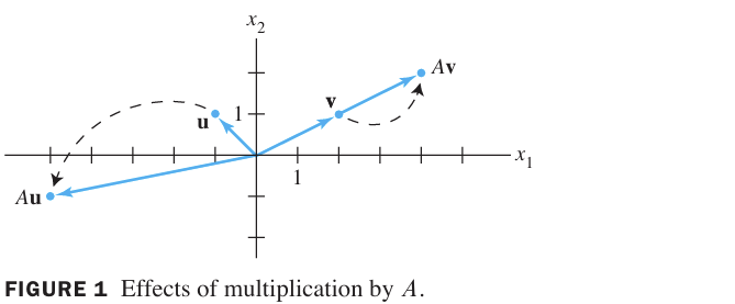
Geometrically, the transformation \(\mathbf{x} \mapsto A\mathbf{x}\) simply stretches (or compresses, or flips) the eigenvector without changing its direction.
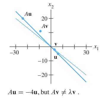
Thus \(\mathbf{v}\) is an eigenvector corresponding to \(\lambda = 2\), but \(\mathbf{u}\) is not an eigenvector because \(A\mathbf u\) is not a multiple of \(\mathbf u\).
(Textbook Figure 1 – horizontal shear and a vector that is merely stretched.)
Note that the columns are obviously linearly dependent, so \((A - 7 I)\mathbf{x} = \mathbf{0}\) has nontrivial solutions. Thus \(7\) is an eigenvalue of \(A\).
Part 2: Row reduce the augmented matrix for \((A-7I)\mathbf{x} = \mathbf{0}\):
The general solution is \(x_1 = x_2\), \(x_2\) free.
So eigenvectors are all multiples of \(\begin{bmatrix} 1 \\ 1 \end{bmatrix}\), i.e., in the form of \(x_2\begin{bmatrix} 1 \\ 1 \end{bmatrix}\). Thus, each vector of this form with \(x_2\neq 0\) is an eigenvector corresponding to \(\lambda =7\).
N.B. The eigenspace for \(\lambda=7\) is the line spanned by \((1,1)\), that can be denoted by \(\{t\begin{bmatrix} 1 \\ 1 \end{bmatrix}, t\in \mathbb R\}\), that is, \[\operatorname{Nul}(A-\lambda I)=\operatorname{Span}\{\begin{bmatrix}1\\1\end{bmatrix}\}\]
Eigenspace
The eigenspace of \(A\) corresponding to an eigenvalue \(\lambda\) is the null space of \(A - \lambda I\): \[\operatorname{Nul}(A - \lambda I) = \{\mathbf{x} \mid (A - \lambda I)\mathbf{x} = \mathbf{0}\}.\] It consists of all eigenvectors for \(\lambda\), together with the zero vector.
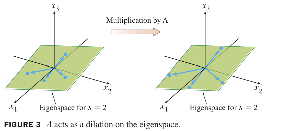
Example 4 (textbook). For \(A = \begin{bmatrix} 4 & -1 & 6 \\ 2 & 1 & 6 \\ 2 & -1 & 8 \end{bmatrix}\), \(\lambda = 2\) is an eigenvalue. Find a basis for the eigenspace.
\[\mathbf{v}_1 = \begin{bmatrix} 1/2 \\ 1 \\ 0 \end{bmatrix},\; \mathbf{v}_2 = \begin{bmatrix} -3 \\ 0 \\ 1 \end{bmatrix}.\]
Thus the eigenspace is two‑dimensional (a plane through the origin).
Eigenvalues of Triangular Matrices
Theorem 1
Theorem 1.
The eigenvalues of a triangular matrix are the entries on its main diagonal.
Proof Outline (for simplicity, we use the example of upper triangular case\(3 \times 3\)):
Set up the characteristic matrix:
If \(A\) is upper triangular, subtracting \(\lambda I\) leaves it upper triangular: \[ A - \lambda I = \begin{bmatrix} a_{11} - \lambda & a_{12} & a_{13} \\ 0 & a_{22} - \lambda & a_{23} \\ 0 & 0 & a_{33} - \lambda \end{bmatrix}. \]
Apply the eigenvalue criterion:
By definition, \(\lambda\) is an eigenvalue of \(A\)\[ \iff (A - \lambda I)x = 0 \text{ has a nontrivial solution} \]\[ \iff A - \lambda I \text{ is not invertible}. \]
Connect to the determinant and Compute the determinant:
From the Invertible Matrix Theorem, a matrix is not invertible \[ \lambda \text{ is an eigenvalue of } A \iff \det(A - \lambda I) = 0. \]
Since \(A - \lambda I\) is triangular, its determinant is simply the product of its diagonal entries: \[\det(A - \lambda I) = (a_{11} - \lambda)(a_{22} - \lambda)(a_{33} - \lambda). \]
Conclude:
Setting this equal to zero gives: \[ (a_{11} - \lambda)(a_{22} - \lambda)(a_{33} - \lambda) = 0. \] By the zero-product property, this happens \[ \iff \lambda = a_{11},\ \lambda = a_{22},\ \text{or } \lambda = a_{33}. \] Hence, the eigenvalues are precisely the diagonal entries of \(A\).
Comments:
For the general triangular matrix of\(n \times n\) case, the same logic applies: the determinant is \(\prod_{i=1}^n (a_{ii} - \lambda)\), which is zero exactly when \(\lambda\) matches one of the diagonal entries.
The proof for lower triangular matrices follows the same logic using forward substitution.
Example 5 (textbook.) \(A = \begin{bmatrix} 3 & 6 & -8 \\ 0 & 0 & 6 \\ 0 & 0 & 2 \end{bmatrix}\) is upper triangular, so by Theorem 1, its eigenvalues are 3, 0, and 2. \(B = \begin{bmatrix} 4 & 0 & 0 \\ -2 & 1 & 0 \\ 5 & 3 & 4 \end{bmatrix}\) is lower triangular, so its eigenvalues are the diagonal entries: 4 and 1 (note that 4 has algebraic multiplicity 2).
Key Insight: The Meaning of Zero Eigenvalues
If \(0\) is an eigenvalue of a matrix \(A\), then there exists a nonzero vector \(x\) such that: \[ Ax = 0x \quad \Longleftrightarrow \quad Ax = 0 \]
The equation \(Ax = 0\) has a nontrivial solution if and only if the matrix \(A\) is not invertible (singular).
Therefore, we conclude the important equivalence:
\(0\) is an eigenvalue of \(A\)\(\quad \Longleftrightarrow \quad\)\(A\) is not invertible.
N.B. This fact is later added to the Invertible Matrix Theorem.
Linearly Independent Eigenvectors
Theorem 2
Theorem 2.
If \(\mathbf{v}_1, \dots, \mathbf{v}_r\) are eigenvectors corresponding to distinct eigenvalues \(\lambda_1, \dots, \lambda_r\) of an \(n\times n\) matrix \(A\), then the set \(\{\mathbf{v}_1, \dots, \mathbf{v}_r\}\) is linearly independent.
This result is crucial for diagonalization (Section 5.3).
Proof (by Contradiction):
Assume dependence & pick the “first” dependent vector:
Suppose the set is linearly dependent. Since \(\mathbf{v}_1 \neq \mathbf{0}\), there exists a first vector \(\mathbf{v}_{p+1}\) that is a linear combination of the preceding vectors \(\mathbf{v}_1, \dots, \mathbf{v}_p\) (Section 1.7 Theorem 7). By choosing the first such vector, we guarantee that \(\{\mathbf{v}_1, \dots, \mathbf{v}_p\}\) is linearly independent.
Write the linear combination: There exist scalars \(c_1, \dots, c_p\) such that \[ \mathbf{v}_{p+1} = c_1\mathbf{v}_1 + \cdots + c_p\mathbf{v}_p. \tag{1} \]
Apply the matrix\(A\) to both sides:
Using \(A\mathbf{v}_k = \lambda_k \mathbf{v}_k\), we get \[ \lambda_{p+1}\mathbf{v}_{p+1} = c_1\lambda_1\mathbf{v}_1 + \cdots + c_p\lambda_p\mathbf{v}_p. \tag{2} \]
Eliminate\(\mathbf{v}_{p+1}\):
Multiply equation (1) by \(\lambda_{p+1}\) and subtract it from equation (2). This cancels the left-hand side, leaving: \[ \mathbf{0} = c_1(\lambda_1 - \lambda_{p+1})\mathbf{v}_1 + \cdots + c_p(\lambda_p - \lambda_{p+1})\mathbf{v}_p. \tag{3} \]
Use independence of\(\{\mathbf{v}_1, \dots, \mathbf{v}_p\}\):
Since these vectors are linearly independent, all coefficients in (3) must be zero: \[ c_i(\lambda_i - \lambda_{p+1}) = 0 \quad \text{for all } i = 1, \dots, p. \]
Reach the contradiction:
The eigenvalues are distinct, so \(\lambda_i \neq \lambda_{p+1}\) for every \(i\). Hence \(c_i = 0\) for all \(i\). Plugging this back into (1) gives \[ \mathbf{v}_{p+1} = \mathbf{0}, \]
which is impossible because an eigenvector is never the zero vector.
Conclusion:
Our assumption of linear dependence must be false. Therefore, \(\{\mathbf{v}_1, \dots, \mathbf{v}_r\}\) is linearly independent.
Section 5.2 The Characteristic Equation
Learning Objectives
After this lecture you will be able to:
State the definition of the characteristic polynomial and use it to determine eigenvalues and their algebraic multiplicities.
Explain why similar matrices have the same characteristic polynomial (and thus the same eigenvalues).
Use eigenvectors and eigenvalues to write explicit formulas for discrete dynamical systems.
Theoretical Foundation: Computing Determinants via Row Reduction
For an \(n \times n\) matrix \(A\), let \(U\) be any echelon form obtained from \(A\) using only row replacements and row interchanges (i.e., withoutscaling rows). Let \(r\) be the number of row interchanges performed.
Then the determinant is defined as: \[ \det A = (-1)^r \cdot (u_{11} \cdot u_{22} \cdots u_{nn}) \] where \(u_{ii}\) are the diagonal entries of \(U\).
Important notes regarding invertibility:
If \(A\) is invertible, all diagonal entries \(u_{ii}\) are pivots (non-zero).
If \(A\) is not invertible, at least the last diagonal entry \(u_{nn}\) is zero, making the product zero.
Thus, we can write: \[ \det A = \begin{cases} (-1)^r \cdot \left( \text{product of pivots in } U \right), & \text{if } A \text{ is invertible} \\[6pt] 0, & \text{if } A \text{ is not invertible} \end{cases} \tag{1} \]
N.B. The determinant is independent of the specific row reduction path chosen—as long as we correctly count row interchanges and never scale rows.
Example 2 (textbook). Compute \(\det A\) for \[ A = \begin{bmatrix} 1 & 5 & 0 \\ 2 & 4 & -1 \\ 0 & -2 & 0 \end{bmatrix}. \]
1. Start from the same first step: \[ A \sim \begin{bmatrix} 1 & 5 & 0 \\ 0 & -6 & -1 \\ 0 & -2 & 0 \end{bmatrix} \] 2. Eliminate below the second pivot by adding \(-\frac{1}{3}R_2\) to \(R_3\) (no interchange, so \(r=0\)): \[ \sim \begin{bmatrix} 1 & 5 & 0 \\ 0 & -6 & -1 \\ 0 & 0 & \frac{1}{3} \end{bmatrix} = U_2 \] 3. Compute the determinant: \[ \det A = (-1)^0 \cdot (1)(-6)\left(\frac{1}{3}\right) = -2. \]
Both methods yield \(-2\), verifying that the determinant is independent of the elimination path.
Linking Determinants to Eigenvalues: The Characteristic Equation
Definition
For any \(n\times n\) matrix \(A\), the determinant \(\det(A - \lambda I)\) is a polynomial of degree \(n\) in \(\lambda\), called the characteristic polynomial. The equation \[\det(A - \lambda I) = 0\] is the characteristic equation. Its roots are the eigenvalues of \(A\) (counting multiplicities).
Recall that a scalar \(\lambda\) is an eigenvalue of \(A\)if and only if the matrix \(A - \lambda I\) is not invertible (i.e., \((A - \lambda I)\mathbf{x} = \mathbf{0}\) has a nontrivial solution).
From Section 1, a matrix is non-invertible precisely when its determinant is zero. Therefore: \[ \boxed{\lambda \text{ is an eigenvalue of } A \iff \det(A - \lambda I) = 0.} \]
Example 1 (textbook). Find the eigenvalues of \(A = \begin{bmatrix} 2 & 3 \\ 3 & -6 \end{bmatrix}\).
Idea: Find all scalars such that the matrix equation \((A - \lambda I)\mathbf x = \mathbf 0\). This problem is equivalent to finding all \(\lambda\) such that the matrix \(A-\lambda I\) is not invertible, which is exactly when its determinant is zero.
Because the determinant of a triangular matrix is the product of its diagonal entries: \[ \det(A - \lambda I) = (5-\lambda)(3-\lambda)(5-\lambda)(1-\lambda). \]
Hence, the characteristic equation is: \[ (5-\lambda)^2 (3-\lambda)(1-\lambda) = 0, \] or equivalently (by multiplying by \((-1)^4\) to make leading coefficients positive): \[ (\lambda - 5)^2 (\lambda - 3)(\lambda - 1) = 0. \]
Eigenvalues: The diagonal entries are \(5, 3, 5, 1\).
So the eigenvalues are \(5, 3, 5, 1\) (i.e., distinct values \(5, 3, 1\), but 5 appears twice).
N.B. This confirms the earlier theorem: the eigenvalues of a triangular matrix are precisely its diagonal entries.
N.B. In Example 3, the eigenvalue \(5\) has multiplicity\(2\), while \(3\) and \(1\) each have multiplicity \(1\).
Algebraic Multiplicity of Eigenvalues
When an eigenvalue appears multiple times as a root of the characteristic polynomial, we assign it a multiplicity.
Definition:
The (algebraic) multiplicity of an eigenvalue \(\lambda\) is the number of times\((\lambda - \lambda_0)\) appears as a factor in the characteristic polynomial (i.e., its multiplicity as a root of the characteristic equation).
Example 4 (textbook) - Finding Eigenvalues and Multiplicities. The characteristic polynomial of a \(6 \times 6\) matrix is \[ \lambda^6 - 4\lambda^5 - 12\lambda^4. \]
Find the eigenvalues and their algebraic multiplicities.
Set the characteristic equation equal to zero: \[ \lambda^4 (\lambda - 6)(\lambda + 2) = 0. \]
Thus, the eigenvalues are:
\(0\) (multiplicity \(4\)),
\(6\) (multiplicity \(1\)),
\(-2\) (multiplicity \(1\)).
N.B. Since the matrix is \(6 \times 6\), the sum of all multiplicities is \(4 + 1 + 1 = 6\), which matches the degree of the polynomial. Listed with repetitions: the eigenvalues are \(0, 0, 0, 0, 6, -2\).
Theorem 3 - Properties of Determinant (from Section 3.2)
To compute \(\det(A - \lambda I)\) effectively, we need the key properties:
Let \(A\) and \(B\) be \(n\times n\) matrices,
\(\det A \neq 0\)\(\Longleftrightarrow\)\(A\) invertible,
\(\det(AB) = (\det A)(\det B)\),
\(\det A^T = \det A\),
If \(A\) is triangular, \(\det A\) is the product of entries on the main diagonal,
Row replacement on \(A\) doe not change the determinant; row swap changes the sign of \(\det A\); row scaling multiplies \(\det\) by that scalar.
These properties are essential for theoretical arguments as well as for evaluating \(\det(A-\lambda I)\) by hand.
IMT addition: The number \(0\) is an eigenvalue of \(A\) iff \(\det A = 0\), i.e., \(A\) is not invertible.
Summary of Key Formulas
Concept
Formula
Determinant via elimination
\(\det A = (-1)^r \cdot \prod u_{ii}\)
Characteristic equation
\(\det(A - \lambda I) = 0\)
Eigenvalue condition
\(\lambda\) is an eigenvalue \(\iff \det(A - \lambda I) = 0\)
Algebraic multiplicity
The exponent of \((\lambda - \lambda_0)\) in the characteristic polynomial
Similarity
Definition
A square matrix \(A\) is similar to \(B\) if there exists an invertible \(P\) such that \[P^{-1}AP = B\] or, equivalently, \(A = PBP^{-1}.\)
Writing \(Q\) for \(P^{-1}\), we have \(Q^{-1}BQ=A\). So \(B\) is also similar to \(A\), and we say simply that \(A\)and\(B\)are similar.
Changing \(A\) into \(P^{-1}AP\) is called a similarity transformation.
Theorem 4
Theorem 4.
Similar matrices have the same characteristic polynomial, and therefore the same eigenvalues with the same multiplicities.
Based on the multiplicative property in Theorem 3, \[\det(B - \lambda I) = \det(P^{-1})\det(A - \lambda I)\det(P).\]
Since \(\det(P^{-1})\det(P)=\det(P^{-1}P)=\det(I)=1\),
\[\det(B - \lambda I) = \det(A - \lambda I).\]
Similarity will be central when we diagonalize matrices.
N.B. Similarity is different from row equivalence. Row operations on a matrix usually change its eigenvalues.
Application to Dynamical Systems (Discrete Linear Systems)
The Big Idea
Many real-world processes evolve in discrete time steps: \[ \mathbf{x}_{k+1} = A\mathbf{x}_k, \quad k = 0,1,2,\dots \] where \(\mathbf{x}_k\) is the state vector at time \(k\) and \(A\) is an \(n \times n\) matrix.
If \(A\) has a basis of eigenvectors, we can write the initial state \(\mathbf{x}_0\) as a linear combination of eigenvectors. Then, because eigenvectors evolve independently (each scaled by its eigenvalue each step), we get an explicit closed-form formula for \(\mathbf{x}_k\). This formula reveals the long‑term (steady‑state) behavior immediately.
Example 5 (textbook)-Migration Model / Markov Chain
Let \[ A = \begin{bmatrix} 0.95 & 0.03 \\ 0.05 & 0.97 \end{bmatrix}, \qquad \mathbf{x}_0 = \begin{bmatrix} 0.6 \\ 0.4 \end{bmatrix}. \] Analyze the long‑term behavior of the dynamical system \[ \mathbf{x}_{k+1} = A\mathbf{x}_k, \quad k = 0,1,2,\dots \]
(This matrix is a migration matrix: the entries represent yearly probabilities of moving between city and suburbs.\(\mathbf{x}_k\) gives the population fractions in each region after \(k\) years.)
Check:\(\mathbf{v}_1\) and \(\mathbf{v}_2\) are linearly independent (since they are not multiples), so they form a basis for \(\mathbb{R}^2\). This is guaranteed because they correspond to distinct eigenvalues (Theorem 2).
Step 2 – Express the Initial State in the Eigenvector Basis
We need scalars \(c_1, c_2\) such that \[ \mathbf{x}_0 = c_1\mathbf{v}_1 + c_2\mathbf{v}_2. \]
As \(k \to \infty\), the term \((0.92)^k\) decays to zero because \(|0.92| < 1\). Therefore, \[ \mathbf{x}_k \to 0.125\,\mathbf{v}_1 = 0.125 \begin{bmatrix} 3 \\ 5 \end{bmatrix} = \begin{bmatrix} 0.375 \\ 0.625 \end{bmatrix}. \]
Interpretation:
The system reaches a steady state\(\mathbf{x}_\infty = \begin{bmatrix} 0.375 \\ 0.625 \end{bmatrix}\).
This means that in the long run, 37.5% of the population lives in the city and 62.5% in the suburbs.
Comments:
In Example 5, \(\lambda_1 = 1\) gave the steady state, and \(\lambda_2 = 0.92\) (with magnitude \(<1\)) caused the transient part to die out.
Notice that the steady state is a multiple of the eigenvector corresponding to\(\lambda = 1\). This is typical for Markov chains: the eigenvector for eigenvalue \(1\) (when it exists) is the steady‑state distribution.
Key Observations for Dynamical Systems (Optional):
Condition on eigenvalues
Long‑term behavior of \(\mathbf{x}_k\)
All \(|\lambda_i| < 1\)
\(\mathbf{x}_k \to \mathbf{0}\) (stable, decays to origin)
One eigenvalue \(= 1\), others \(|\lambda_i| < 1\)
\(\mathbf{x}_k\) tends to a non‑zero steady state (a multiple of the eigenvector for \(\lambda = 1\))
Any \(|\lambda_i| > 1\)
\(\mathbf{x}_k\) grows without bound (unstable)
Eigenvalues with \(|\lambda_i| = 1\) but not \(1\)
Oscillatory or periodic behavior (depending on complex eigenvalues)
Connection to Markov Chains (Optional)
The matrix \(A\) in this example is the migration matrix from Section 4.9 of the textbook.
\(\mathbf{x}_k\) is the population distribution after \(k\) years.
The columns of \(A\) sum to 1 (a stochastic matrix), so \(\lambda = 1\) is always an eigenvalue.
The steady‑state vector is precisely the eigenvector for \(\lambda = 1\), scaled so that its entries sum to 1.
Summary of the Solution Method
To analyze \(\mathbf{x}_{k+1} = A\mathbf{x}_k\):
Find eigenvalues and eigenvectors of \(A\).
Expressthe initial state\(\mathbf{x}_0\) as a linear combination of eigenvectors (in the eigenvector basis): \(\mathbf{x}_0 = c_1\mathbf{v}_1 + \cdots + c_n\mathbf{v}_n\).
Take the limit\(k \to \infty\) to determine long‑term behavior. The eigenvalues with magnitude \(<1\) vanish; those with magnitude \(>1\) cause growth; \(\lambda = 1\) (if present) gives the steady state.
This powerful technique turns a recursive system into a simple algebraic formula, revealing the full trajectory at a glance.
Practice Problems (in‑class)
Determine if \(\mathbf{v} = \begin{bmatrix} 4 \\ -3 \end{bmatrix}\) is an eigenvector of \(A = \begin{bmatrix} 5 & 8 \\ -4 & -7 \end{bmatrix}\). If so, find the eigenvalue.
Find the eigenvalues of \(A = \begin{bmatrix} 3 & -2 \\ 1 & -1 \end{bmatrix}\) using the characteristic equation.
For \(A\) in Problem 2, find a basis for the eigenspace corresponding to each eigenvalue.
Let \(A = \begin{bmatrix} 2 & 1 \\ -1 & 4 \end{bmatrix}\). Compute the characteristic polynomial. What are the eigenvalues and their algebraic multiplicities? (Hint: the characteristic polynomial is \(\lambda^2 - 6\lambda + 9\); what does this tell you about the eigenvalues?)
Suppose \(A\) is similar to \(B\). If \(A\) has eigenvalues \(3\) and \(-2\), what are the eigenvalues of \(B\)?
Consider the dynamical system \(\mathbf{x}_{k+1} = A\mathbf{x}_k\) with \(A = \begin{bmatrix} 1 & 2 \\ 2 & 1 \end{bmatrix}\) and \(\mathbf{x}_0 = \begin{bmatrix} 1 \\ 0 \end{bmatrix}\). Find the eigenvalues and eigenvectors of \(A\). Write an explicit formula for \(\mathbf{x}_k\). (You do not need to compute the exact coefficients; outline the method.)
(Solutions at the end.)
R Supplement
# Eigenvalues and eigenvectors using built-in functionA <-matrix(c(3, -2, 1, 0), nrow=2)eigen(A)$values
# Verifying eigenspace: solve (A - lambda*I) x = 0lambda <-7A_ex <-matrix(c(1,5,6,2), nrow=2)A_minus <- A_ex - lambda *diag(2)# Row reduce to find null space basislibrary(pracma)rref(cbind(A_minus, c(0,0)))
     [,1] [,2] [,3]
[1,]    1   -1    0
[2,]    0    0    0
# Characteristic polynomial via det(A - lambda*I) symbolically hard, but we can evaluate for given lambda# For a 2x2 we can compute coefficients directlyA2 <-matrix(c(2,3,3,-6), nrow=2)poly <-function(lambda) det(A2 - lambda*diag(2))# Find roots manually? Use uniroot or optim, but eigen gives exact eigenvalues.eigen(A2)$values
Compute \(A\mathbf{v} = \begin{bmatrix} 5(4)+8(-3) \\ -4(4) -7(-3) \end{bmatrix} = \begin{bmatrix} -4 \\ 5 \end{bmatrix}\). Is this a scalar multiple of \((4,-3)\)? No, so \(\mathbf{v}\) is not an eigenvector.
We already found the eigenvalues \(\lambda_1 = 1+\sqrt2,\lambda_2 = 1-\sqrt2.\) For each eigenvalue, the eigenspace is the nullspace of \(A - \lambda I\). We solve \((A - \lambda I)\mathbf{x} = \mathbf{0}\).
Row Reduction: Swap rows to get a leading 1 and eliminate the entry below the pivot. \[ R_1 \leftrightarrow R_2 \quad\longrightarrow\quad \begin{bmatrix} 1 & -2-\sqrt2 \\ 2-\sqrt2 & -2 \end{bmatrix} \] \[ R_2 \rightarrow R_2 - (2-\sqrt2)R_1 \] So we get a free variable: \[ \begin{bmatrix} 1 & -2-\sqrt2 \\ 0 & 0 \end{bmatrix} \]
Now the equation is: \[ x_1 + (-2-\sqrt2)x_2 = 0 \quad\Rightarrow\quad x_1 = (2+\sqrt2)x_2. \]
Choose \(x_2 = 2-\sqrt2\) to avoid radicals in the first component: \[ x_1 = (2+\sqrt2)(2-\sqrt2) = 4 - 2 = 2. \] So a nonzero eigenvector is \[ \mathbf{v}_1 = \begin{bmatrix} 2 \\ 2-\sqrt2 \end{bmatrix}. \]
Therefore, the eigenspace for \(\lambda_1 = 1+\sqrt2\) is \[ E_{1+\sqrt2} = \operatorname{span}\left\{ \begin{bmatrix} 2 \\ 2-\sqrt2 \end{bmatrix} \right\}, \] and a basis is given by the single vector \(\left\{\begin{bmatrix} 2 \\ 2-\sqrt2 \end{bmatrix}\right\}\).
Step 3: Compute \(c_1,c_2\) from \(\mathbf{x}_0 = (1,0)\): solving gives \(c_1=c_2=1/2\). So \[\mathbf{x}_k = \frac12 (3^k \begin{bmatrix}1\\1\end{bmatrix} + (-1)^k \begin{bmatrix}1\\-1\end{bmatrix}).\]
Summary
Eigenvectors are vectors whose direction is unchanged by \(A\) (merely scaled).
Eigenvalues are scalars \(\lambda\) for which \(A-\lambda I\) is singular.
The characteristic equation \(\det(A-\lambda I)=0\) provides a polynomial whose roots are the eigenvalues.
Algebraic multiplicities describe how many times an eigenvalue is a root.
Eigenspaces are null spaces of \(A-\lambda I\).
Similar matrices share the same characteristic polynomial.
Linear combinations of eigenvectors give explicit solutions to dynamical systems.
Sections 5.3 Diagonalization
Learning Objectives
After this lecture you will be able to:
Diagonalize a matrix by finding an invertible matrix \(P\) and a diagonal matrix \(D\) such that \(A = PDP^{-1}\).
Compute powers of a diagonalizable matrix using \(A^k = PD^kP^{-1}\).
Determine whether a matrix is diagonalizable using the Diagonalization Theorem.
Apply the condition that an \(n\times n\) matrix with \(n\) distinct eigenvalues is diagonalizable.
Understand the geometric meaning of diagonalization as a change of basis to an eigenvector basis.
Motivation: Why Diagonalization Matters
In many applications, we need to compute high powers of a matrix \(A\), such as \(A^k\) for large \(k\). Direct multiplication is inefficient.
However, a diagonal matrix is easy to work with: powers, determinants, eigenvalues are all simple. If a matrix \(A\) is similar to a diagonal matrix\(D\), i.e., if we can factor \(A\) as
\[A = PDP^{-1}\]
for some invertible \(P\), then many computations become easy through the similarity relation.
A square matrix \(A\) is diagonalizable if it is similar to a diagonal matrix, i.e., there exists an invertible matrix \(P\) and a diagonal matrix \(D\) such that: \[A = PDP^{-1}.\]
Theorem 5 (Diagonalization Theorem).
An \(n\times n\) matrix \(A\) is diagonalizable if and only if \(A\) has \(n\) linearly independent eigenvectors.
In fact, \(A = PDP^{-1}\) with \(D\) diagonal if and only if the columns of \(P\) are \(n\) linearly independent eigenvectors of \(A\). The diagonal entries of \(D\) are the corresponding eigenvalues.
In other words, \(A\) is diagonalizable if and only if there are enough eigenvectors to form a basis of \(\mathbb{R}^n\). Such a basis is called an eigenvector basis.
Proof outline:\(AP = PD\) means that each column \(\mathbf{v}_j\) of \(P\) satisfies \(A\mathbf{v}_j = \lambda_j \mathbf{v}_j\). If the \(\mathbf{v}_j\) are also linearly independent, \(P\) is invertible and we can write \(A = PDP^{-1}\).
Proof.
We prove both directions.
Step 1: Preliminary Observation
Let \(P\) have columns \(\mathbf{v}_1, \dots, \mathbf{v}_n\), and let any diagonal matrix \[D = \begin{bmatrix} \lambda_1 & 0 & \cdots & 0 \\ 0 & \lambda_2 & \cdots & 0 \\ \vdots & \vdots & \ddots & \vdots \\ 0 & 0 & \cdots & \lambda_n \end{bmatrix}.\]
Right side: \[PD = [\lambda_1\mathbf{v}_1 \ \cdots \ \lambda_n\mathbf{v}_n].\]
Thus: \[AP = PD \quad \Longleftrightarrow \quad A\mathbf{v}_i = \lambda_i \mathbf{v}_i \text{ for each } i.\]
Step 2: Only If Direction (\(A\) Diagonalizable \(\Rightarrow\) n Independent Eigenvectors)
Assume \(A = PDP^{-1}\). Then right-multiplying by \(P\): \[AP = PD.\]
By the observation above: \[A\mathbf{v}_i = \lambda_i \mathbf{v}_i \quad \text{for each } i.\]
Since \(P\) is invertible, its columns \(\mathbf{v}_1, \dots, \mathbf{v}_n\) are linearly independent. Also, since eigenvectors are nonzero by definition, each \(\lambda_i\) is an eigenvalue of \(A\). Thus \(A\) has \(n\) linearly independent eigenvectors.
Step 3: If Direction (n Independent Eigenvectors \(\Rightarrow\) Diagonalizable)
Since the eigenvectors are linearly independent, \(P\) is invertible. By the observation: \[AP = PD.\]
Right-multiply by \(P^{-1}\): \[A = PDP^{-1}.\]
Thus \(A\) is diagonalizable. \(\square\)
Diagonalization Procedure (Step-by-Step)
To diagonalize an \(n \times n\) matrix \(A\) (if possible):
Step 1: Find the eigenvalues of \(A\) by solving \(\det(A - \lambda I) = 0\).
Step 2: For each eigenvalue, find a basis for its eigenspace (i.e., find the eigenvectors). If the total number of linearly independent eigenvectors found is less than \(n\), then \(A\) is not diagonalizable.
Step 3: Form the matrix \(P\) whose columns are the \(n\) linearly independent eigenvectors.
Step 4: Form the diagonal matrix \(D\) whose diagonal entries are the corresponding eigenvalues, in the same order as the eigenvectors in \(P\).
Verification: Check that \(AP = PD\) (this avoids computing \(P^{-1}\)).
Example 4 (textbook – not diagonalizable).\(A = \begin{bmatrix} 2 & 4 & 3 \\ -4 & -6 & -3 \\ 3 & 3 & 1 \end{bmatrix}\) has the same characteristic equation as Example 3, but each eigenspace is only one‑dimensional. Only two linearly independent eigenvectors exist, so \(A\) is not diagonalizable.
Example 4 (textbook - Non-Diagonalizable Matrix) Diagonalize, if possible \[A = \begin{bmatrix} 2 & 4 & 3 \\ -4 & -6 & -3 \\ 3 & 3 & 1 \end{bmatrix}.\]
Solution:
The characteristic polynomial is the same as Example 3: \[\det(A - \lambda I) = -(\lambda - 1)(\lambda + 2)^2.\]
So eigenvalues are \(\lambda = 1\) and \(\lambda = -2\) (multiplicity 2).
Total linearly independent eigenvectors = \(2 < 3\).
Since each eigenspace is only one‑dimensional. Only two linearly independent eigenvectors exist, so \(A\) is not diagonalizable (by theorem 5).
Theorem 6 - Distinct eigenvalues and diagonalizability
Theorem 6
An \(n\times n\) matrix with \(n\)distinct eigenvalues is diagonalizable.
N.B. Theorem is a sufficient condition for diagonalizability.
N.B. This condition is sufficient but not necessary. Example 3 has only two distinct eigenvalues but is still diagonalizable.
Proof.
Eigenvectors corresponding to distinct eigenvalues are linearly independent (Theorem 2, Section 5.1). Thus we have \(n\) linearly independent eigenvectors (forming a basis). By Theorem 5, \(A\) is diagonalizable.
Example 5 (textbook). Is the following matrix \[A = \begin{bmatrix} 5 & -8 & 1 \\ 0 & 0 & 7 \\ 0 & 0 & -2 \end{bmatrix}\] diagonalizable?
Solution.
Since \(A\) is triangular, its eigenvalues are the diagonal entries: \(5, 0, -2\). These are three distinct eigenvalues for a \(3 \times 3\) matrix. By Theorem 6, \(A\) is diagonalizable.
The General Case: Repeated Eigenvalues
When eigenvalues are not distinct (or repeated), i.e., an \(n \times n\) matrix \(A\) has less than \(n\) distinct eigenvalues, it is still possible to build \(P\). Diagonalizability depends on the dimension of the eigenspace (the geometric multiplicity).
Theorem 7
Theorem 7
Let \(A\) be an \(n \times n\) matrix with distinct eigenvalues \(\lambda_1, \dots, \lambda_p\).
For each \(1\leq k\leq p\), the dimension of the eigenspace for \(\lambda_k\) is at most the multiplicity of \(\lambda_k\).
\(A\) is diagonalizableif and only if the sum of the dimensions of the eigenspaces equals\(n\). This happens if and only if:
The characteristic polynomial factors completely into linear factors, and
The dimension of each eigenspace equals the multiplicity of its eigenvalue.
If \(A\) is diagonalizable, then the union of bases for the eigenspaces forms an eigenvector basis for \(\mathbb{R}^n\).
Interpretation: The matrix is diagonalizable iff the sum of the dimensions of the eigenspaces equals \(n\), which happens exactly when the geometric multiplicity equals the algebraic multiplicity for each eigenvalue.
Key Insight:
The geometric multiplicity (dimension of eigenspace) must equal the algebraic multiplicity (multiplicity as a root of the characteristic polynomial) for each eigenvalue.
If any eigenspace has dimension less than its eigenvalue’s multiplicity, the matrix is not diagonalizable.
Idea: the matrix has eigenvalues \(5\) and \(-3\), each multiplicity 2. The eigenspaces are both two‑dimensional, so \(A\) is diagonalizable. We can construct \(P\) and \(D\) accordingly.
Solution:
Since \(A\) is triangular, the eigenvalues are the diagonal entries: \[\lambda = 5 \text{ (multiplicity 2)}, \quad \lambda = -3 \text{ (multiplicity 2)}.\]
Diagonalize \(A = \begin{bmatrix} 1 & 0 \\ 6 & -1 \end{bmatrix}\) if possible. If it is diagonalizable, give \(P\), \(D\), and \(P^{-1}\).
Compute \(A^4\) for \(A = \begin{bmatrix} 4 & -3 \\ 2 & -1 \end{bmatrix}\) given that \(A = PDP^{-1}\) with \(P = \begin{bmatrix} 3 & 1 \\ 2 & 1 \end{bmatrix}\), \(D = \begin{bmatrix} 2 & 0 \\ 0 & 1 \end{bmatrix}\). (Hint: find \(P^{-1}\) and use \(A^4 = PD^4 P^{-1}\).)
Determine if \(A = \begin{bmatrix} 4 & 2 & 2 \\ 2 & 4 & 2 \\ 2 & 2 & 4 \end{bmatrix}\) is diagonalizable. Its eigenvalues are \(2\) (multiplicity 2) and \(8\). (Hint: Check if the eigenspace for \(\lambda = 2\) is two‑dimensional.)
(Solutions at the end.)
R Supplement
# Diagonalization example 2A <-matrix(c(7, -4, 2, 1), nrow=2)eig <-eigen(A)P <- eig$vectorsD <-diag(eig$values)P %*% D %*%solve(P) # should equal A
     [,1] [,2]
[1,]    7    2
[2,]   -4    1
# Compute A^8 using diagonalizationk <-8A_pow <- P %*%diag(eig$values^k) %*%solve(P)A_pow
        [,1]    [,2]
[1,]  774689  384064
[2,] -768128 -377503
# Check if a matrix is diagonalizable (by checking eigenvectors)A3 <-matrix(c(4,2,2, 2,4,2, 2,2,4), nrow=3)eig3 <-eigen(A3)eig3$values
[1] 8 2 2
P3 <- eig3$vectors# Check if P3 is invertible (determinant != 0)det(P3) # if nonzero, diagonalizable
[1] -1
# B-matrix of differentiation on P_2# Basis B = {1, t, t^2}; T(p)=p'# T(1)=0, T(t)=1, T(t^2)=2t => coordinate vectorsMB <-matrix(c(0,0,0, 1,0,0, 0,2,0), nrow=3, byrow=TRUE)MB
\(A\) is symmetric (real symmetric matrices are diagonalizable, but we haven’t proved that yet).
Check eigenspaces:
For \(\lambda=2\), solve \((A-2I)\mathbf{x}=\mathbf{0}\). \(A-2I = \begin{bmatrix}2&2&2\\2&2&2\\2&2&2\end{bmatrix} \sim \begin{bmatrix}1&1&1\\0&0&0\\0&0&0\end{bmatrix}\). Two free variables → eigenspace dimension 2 (multiplicity 2).
For \(\lambda=8\), dimension 1.
Total \(1+2=3\) = size, so \(A\) is diagonalizable.
Summary
A matrix is diagonalizable if it has a full set of \(n\) linearly independent eigenvectors.
\(A = PDP^{-1}\) with \(D\) diagonal gives easy computation of powers and long‑term behavior.
Distinct eigenvalues guarantee diagonalizability; repeated eigenvalues may still allow diagonalization if geometric multiplicity equals algebraic multiplicity.
Diagonalization corresponds to choosing a basis of eigenvectors: the linear transformation then acts as simple scaling along each basis direction. (section 5.4)
The matrix of a linear transformation with respect to a basis captures the transformation’s action in coordinates. (section 5.4)
These notes follow Chapter 5 of Lay, Lay & McDonald, “Linear Algebra and its Applications”, 5th edition.